Summary#
import os
# os.chdir('path/to/book/directory')
os.chdir('..')
import sys
from pathlib import Path
sys.path.append(str(Path.cwd()))
from src.ci_adapt_utilities import *
import matplotlib.pyplot as plt
import math

data_path = Path(os.getcwd() + '/data')
interim_data_path = data_path / 'interim' / 'collected_flood_runs'
Load default configuration and model parameters
config_file=Path(os.getcwd() + '/config_ci_adapt_test.ini')
hazard_type, infra_type, country_code, country_name, hazard_data_subfolders, asset_data, vulnerability_data = load_config(config_file)
Define paths for adaptations, basins, and region (for visualisation)
adaptations_df_dir = data_path / 'interim' / 'adaptations'
basins_path = data_path / 'Floods' / 'basins' / 'hybas_eu_lev01-12_v1c' / 'hybas_eu_lev08_v1c_valid.shp'
regions_path = data_path / Path('visualisation/rhineland_palatinate.geojson')

regions_gdf = gpd.read_file(regions_path)
basins_gdf_0 = load_basins_in_region(basins_path, regions_path, clipping=True)
basin_list_tributaries, basin_list_full_flood = find_basin_lists(basins_gdf_0)
Load asset data, adaptation cost data, and results from baseline (no adaptation) risk and adapted risk (with adaptations)
assets, geom_dict, miraca_colors, return_period_dict, adaptation_unit_costs, rp_spec_priority, average_road_cost_per_ton_km, average_train_cost_per_ton_km, average_train_load_tons = startup_ci_adapt(data_path, config_file, interim_data_path)
shortest_paths, disrupted_edges_by_basin, graph_r0, disrupted_shortest_paths, event_impacts, full_flood_event, all_disrupted_edges, collect_output = load_baseline_impact_assessment(data_path)
675 assets loaded.
Loaded data from baseline impact assessment
event_impacts = {haz_map: event_impacts[haz_map] if haz_map in event_impacts.keys() else 0.0 for haz_map in collect_output.keys()}
direct_damages_baseline_sum = {haz_map: (sum(v[0] for v in collect_output[haz_map].values()), sum(v[1] for v in collect_output[haz_map].values())) for haz_map in collect_output}
# Find basins that have damaged assets
overlay_files = [file for file in os.listdir(interim_data_path) if file.endswith('.pkl') and file.startswith('overlay')]
basins_list = list(set([int(file.split('.')[0].split('_')[-1]) for file in overlay_files]))
Define some tag names for clarity in output
dict_tags_names = {'l1': 'L1: flood wall',
                    'l2': 'L2: elevate rail (viaduct)',
                    'l3': 'L3: build new connection',
                    'l4': 'L4: reduce demand',
                    'trib': 'Study Area 2',
                    'rhine': 'Study Area 1',
                    'baseline': 'No adaptation',
                    'upper bound': 'Future C (discounted)',
                    'lower bound': 'Future A (discounted)',
                    'mean': 'Future B (discounted)'}
Calculate the return period frequencies under climate change and define discount rate for future damages discounting
increase_factors_bounds = {'lower bound':{'_H_': 2, '_M_': 1.75, '_L_': 1.82},
                            'mean':{'_H_': 2, '_M_': 4.21, '_L_': 5.86},
                            'upper bound':{'_H_': 2, '_M_': 6.67, '_L_': 9.09}}
num_years = 100
# return_period_dict = {'_H_': 10,'_M_': 100,'_L_': 200} # initial return periods for the different hazard maps
dynamic_rps={inc_f:calculate_dynamic_return_periods(return_period_dict, num_years, increase_factors_bounds[inc_f]) for inc_f in increase_factors_bounds.keys()}
discount_rate_percent = 1 # (Define discounting rate for future benefits)
Calculate future damages under climate change without adaptation (baseline)
#Calculate baseline results for future conditions
adapt_id='baseline'

baseline_results_dict = {}
eadD_bl_by_ts_basin_incf = {}
eadIT_bl_by_ts_basin_incf = {}

direct_damages_adapted, indirect_damages_adapted, indirect_damages_adapted_full, adapted_assets, adaptation_costs, adaptations_df = load_adaptation_impacts(adapt_id, data_path)
total_damages_adapted_df_mill=process_raw_adaptations_output(direct_damages_baseline_sum, direct_damages_adapted, event_impacts, indirect_damages_adapted, adaptations_df)

for inc_f in increase_factors_bounds.keys():
    return_periods = dynamic_rps[inc_f]

    ead_y0_dd_bl_all, ead_y100_dd_bl_all, total_dd_bl_all, eadD_bl_by_ts_basin_incf[inc_f] = compile_direct_risk(inc_f, return_periods, basins_list, collect_output, total_damages_adapted_df_mill, discount_rate_percent)
    ead_y0_id_bl_all, ead_y100_id_bl_all, total_id_bl_all,  eadIT_bl_by_ts_basin_incf[inc_f] = compile_indirect_risk_tributaries(inc_f, return_periods, basins_list, basin_list_tributaries, collect_output, total_damages_adapted_df_mill, discount_rate_percent)
    ead_y0_id_bl_full, ead_y100_id_bl_full, total_id_bl_full = compile_indirect_risk_full_flood(return_periods, indirect_damages_adapted_full, discount_rate_percent)

    baseline_results_dict[inc_f] = {'ead_y0_dd_bl_all': ead_y0_dd_bl_all, 'ead_y100_dd_bl_all': ead_y100_dd_bl_all, 'total_dd_bl_all': total_dd_bl_all,
                                        'ead_y0_id_bl_all': ead_y0_id_bl_all[0], 'ead_y100_id_bl_all': ead_y100_id_bl_all[0], 'total_id_bl_all': total_id_bl_all[0],
                                        'ead_y0_id_bl_full': ead_y0_id_bl_full, 'ead_y100_id_bl_full': ead_y100_id_bl_full, 'total_id_bl_full': total_id_bl_full}
#Baseline damages and losses by return period
direct_damages_adapted, indirect_damages_adapted, indirect_damages_adapted_full, adapted_assets, adaptation_costs, adaptations_df = load_adaptation_impacts(adapt_id, data_path)
total_damages_adapted_df_mill=process_raw_adaptations_output(direct_damages_baseline_sum, direct_damages_adapted, event_impacts, indirect_damages_adapted, adaptations_df)

total_damages_adapted_df_mill
total_damages_adapted_df_mill['basin'] = total_damages_adapted_df_mill.index
total_damages_adapted_df_mill['basin'] = total_damages_adapted_df_mill['basin'].apply(lambda x: int(x.split('_')[-1]))
total_damages_adapted_df_mill['direct damage baseline avg [M€]'] = (total_damages_adapted_df_mill['direct damage baseline lower [M€]'] + total_damages_adapted_df_mill['direct damage baseline upper [M€]'])/2
total_damages_adapted_df_mill['indirect damage baseline_tributaries [M€]'] = np.where(total_damages_adapted_df_mill['basin'].isin(basin_list_tributaries), total_damages_adapted_df_mill['indirect damage baseline [M€]'], 0)
total_damages_adapted_df_mill_sum = total_damages_adapted_df_mill.groupby(['return_period'], observed=True).sum().reset_index()

# keep only return_period direct damage baseline lower [M€]	direct damage baseline upper [M€]	indirect damage baseline_tributaries [M€]
keep_cols = ['return_period', 'direct damage baseline avg [M€]', 'direct damage baseline lower [M€]', 'direct damage baseline upper [M€]', 'indirect damage baseline_tributaries [M€]']
drop_cols = [col for col in total_damages_adapted_df_mill_sum.columns  if col not in keep_cols]
total_damages_adapted_df_mill_sum.drop(columns=[col for col in drop_cols if col in total_damages_adapted_df_mill_sum.columns], inplace=True)

return_period_keys = {'H': 'flood_DERP_RW_H', 'M': 'flood_DERP_RW_M', 'L': 'flood_DERP_RW_L'}
total_damages_adapted_df_mill_sum['indirect damage baseline_mainstem [M€]'] = [
    full_flood_event[return_period_keys[x.split('_')[-1]]] / 1e6 for x in total_damages_adapted_df_mill_sum['return_period']
]
# turn all values to integers except return_period
for col in total_damages_adapted_df_mill_sum.columns:
    if col != 'return_period':
        total_damages_adapted_df_mill_sum[col] = total_damages_adapted_df_mill_sum[col].apply(lambda x: int(x))
Calculate adaptations under future conditions
# Calculate results for adapted conditions
adaptation_files = [file for file in os.listdir(adaptations_df_dir) if file.endswith('.csv')]
adapt_ids = [file.split('_adaptations')[0] for file in adaptation_files]

adapted_results_dict = {}
adaptation_cost_dict = {}
eadD_ad_by_ts_basin_incf = {}
eadIT_ad_by_ts_basin_incf = {}

for adapt_id in adapt_ids:
    direct_damages_adapted, indirect_damages_adapted, indirect_damages_adapted_full, adapted_assets, adaptation_costs, adaptations_df = load_adaptation_impacts(adapt_id, data_path)
    total_damages_adapted_df_mill=process_raw_adaptations_output(direct_damages_baseline_sum, direct_damages_adapted, event_impacts, indirect_damages_adapted, adaptations_df)
    adaptation_cost_dict[adapt_id] = adaptation_costs

    if adapt_id not in adapted_results_dict.keys():
        adapted_results_dict[adapt_id] = {}
        eadD_ad_by_ts_basin_incf[adapt_id] = {}
        eadIT_ad_by_ts_basin_incf[adapt_id] = {}
    for inc_f in increase_factors_bounds.keys():
        if inc_f not in adapted_results_dict[adapt_id]:
            adapted_results_dict[adapt_id][inc_f] = {}

        return_periods = dynamic_rps[inc_f]

        print(adapt_id, inc_f)

        ead_y0_dd_ad_all, ead_y100_dd_ad_all, total_dd_ad_all, eadD_ad_by_ts_basin_incf[adapt_id][inc_f]  = compile_direct_risk(inc_f, return_periods, basins_list, collect_output, total_damages_adapted_df_mill, discount_rate_percent=discount_rate_percent)
        ead_y0_id_ad_all, ead_y100_id_ad_all, total_id_ad_all, eadIT_ad_by_ts_basin_incf[adapt_id][inc_f] = compile_indirect_risk_tributaries(inc_f, return_periods, basins_list, basin_list_tributaries, collect_output, total_damages_adapted_df_mill, discount_rate_percent=discount_rate_percent)
        ead_y0_id_ad_full, ead_y100_id_ad_full, total_id_ad_full = compile_indirect_risk_full_flood(return_periods, indirect_damages_adapted_full, discount_rate_percent=discount_rate_percent)

        adapted_results_dict[adapt_id][inc_f] = {'ead_y0_dd_ad_all': ead_y0_dd_ad_all, 'ead_y100_dd_ad_all': ead_y100_dd_ad_all, 'total_dd_ad_all': total_dd_ad_all,
                                                'ead_y0_id_ad_all': ead_y0_id_ad_all[0], 'ead_y100_id_ad_all': ead_y100_id_ad_all[0], 'total_id_ad_all': total_id_ad_all[0],
                                                'ead_y0_id_ad_full': ead_y0_id_ad_full, 'ead_y100_id_ad_full': ead_y100_id_ad_full, 'total_id_ad_full': total_id_ad_full}
l3_trib lower bound
l3_trib mean
l3_trib upper bound
l2_trib lower bound
l2_trib mean
l2_trib upper bound
baseline lower bound
baseline mean
baseline upper bound
l4_trib lower bound
l4_trib mean
l4_trib upper bound
l1_trib lower bound
l1_trib mean
l1_trib upper bound
Output discounted future risk
future_risk_df = pd.DataFrame()

risk_components = ['Direct damage [M€]', 'Indirect losses tributaries [M€]', 'Indirect losses mainstem [M€]']
increase_factors = ['lower bound', 'mean', 'upper bound']

future_risk_df['Risk component'] = risk_components
future_risk_df['Year 0 (undiscounted)'] = [(baseline_results_dict['mean']['ead_y0_dd_bl_all'][0]+baseline_results_dict['mean']['ead_y0_dd_bl_all'][1])/2, baseline_results_dict['mean']['ead_y0_id_bl_all'], baseline_results_dict['mean']['ead_y0_id_bl_full']]

for inc_f in increase_factors:
    future_risk_df[dict_tags_names[inc_f]] = [(baseline_results_dict[inc_f]['ead_y100_dd_bl_all'][0]+baseline_results_dict[inc_f]['ead_y100_dd_bl_all'][1])/2, baseline_results_dict[inc_f]['ead_y100_id_bl_all'], baseline_results_dict[inc_f]['ead_y100_id_bl_full']]

# add all components
future_risk_df=future_risk_df.T
future_risk_df['total'] = future_risk_df.sum(axis=1)
future_risk_df=future_risk_df.T
future_risk_df.loc['total', 'Risk component'] = 'Total [M€]'

future_risk_df.index = future_risk_df['Risk component']
future_risk_df.drop(columns=['Risk component'], inplace=True)
future_risk_df.to_csv(data_path / 'output' / 'future_risk_df.csv')
future_risk_df
| Year 0 (undiscounted) | Future A (discounted) | Future B (discounted) | Future C (discounted) | |
|---|---|---|---|---|
| Risk component | ||||
| Direct damage [M€] | 1.680 | 1.153 | 1.844 | 2.480 |
| Indirect losses tributaries [M€] | 0.731 | 0.444 | 0.669 | 0.876 |
| Indirect losses mainstem [M€] | 2.048 | 1.180 | 1.963 | 2.678 |
| Total [M€] | 4.460 | 2.778 | 4.477 | 6.034 |
Calculate total discounted adaptation costs including initial cost and maintenance
# Process adaptation costs and benefits for different levels and incorporate yearly maintenance costs
yearly_maintenance_percent = {'l1': 1.0, 'l2': 1.0, 'l3': 1.0}
maintenance_pc_dict = discount_maintenance_costs(yearly_maintenance_percent, discount_rate_percent, num_years)

processed_adaptation_costs = process_adaptation_costs(adaptation_cost_dict, maintenance_pc_dict)

# Find the avoided damages
avoided_damages_dict = {}
for adapt_id in adapt_ids:
    if adapt_id not in adapted_results_dict:
        continue
    avoided_damages_dict[adapt_id] = {}
    for inc_f in increase_factors_bounds.keys():
        avoided_damages_dict[adapt_id][inc_f] = {}
        for key in baseline_results_dict[inc_f].keys():
            key_ad=key.replace('bl','ad')
            key_diff=key.replace('bl','diff')
            avoided_damages_dict[adapt_id][inc_f][key_diff] = baseline_results_dict[inc_f][key] - adapted_results_dict[adapt_id][inc_f][key_ad]

benefits_dict = {}
for adapt_id in adapt_ids:
    benefits_dict[adapt_id] = {}
    for inc_f in increase_factors_bounds.keys():
        benefits_dict[adapt_id][inc_f] = {}
        total_avoided_damages_y0 = avoided_damages_dict[adapt_id][inc_f]['ead_y0_dd_diff_all'] + avoided_damages_dict[adapt_id][inc_f]['ead_y0_id_diff_all'] + avoided_damages_dict[adapt_id][inc_f]['ead_y0_id_diff_full']
        total_avoided_damages_y100 = avoided_damages_dict[adapt_id][inc_f]['ead_y100_dd_diff_all'] + avoided_damages_dict[adapt_id][inc_f]['ead_y100_id_diff_all'] + avoided_damages_dict[adapt_id][inc_f]['ead_y100_id_diff_full']
        total_avoided_damages_full_period = avoided_damages_dict[adapt_id][inc_f]['total_dd_diff_all'] + avoided_damages_dict[adapt_id][inc_f]['total_id_diff_all'] + avoided_damages_dict[adapt_id][inc_f]['total_id_diff_full']
        benefits_dict[adapt_id][inc_f] = {'total_avoided_damages_y0': total_avoided_damages_y0, 'total_avoided_damages_y100': total_avoided_damages_y100, 'total_avoided_damages_full_period': total_avoided_damages_full_period}
Calculate the benefit to cost ratios for each adaptation under each future conditions and save results
adapt_ids=benefits_dict.keys()
bcr_df = pd.DataFrame()

for adapt_id in adapt_ids:
    for inc_f in increase_factors_bounds.keys():
        total_adaptation_cost = processed_adaptation_costs[adapt_id]
        total_avoided_damages = benefits_dict[adapt_id][inc_f]['total_avoided_damages_full_period']
        bcr = total_avoided_damages / total_adaptation_cost if total_adaptation_cost != 0 else math.nan
        bcr = np.nan_to_num(bcr, nan=0)
        # bcr = bcr if bcr != math.nan else 0
        bcr_mean = bcr.mean()
        total_avoided_damages_mean = total_avoided_damages.mean()
        new_df = pd.DataFrame({(adapt_id,inc_f): [total_adaptation_cost, total_avoided_damages_mean, bcr_mean, total_avoided_damages, bcr]}, index=['total_adaptation_cost', 'total_avoided_damages_mean','bcr_mean', 'total_avoided_damages', 'bcr']).T
        bcr_df = pd.concat([bcr_df, new_df])

adapt_ids_output = ['baseline', 'l1_trib', 'l2_trib','l3_trib','l4_trib']#, 'l1_rhine', 'l2_rhine', 'l3_rhine', 'l4_rhine']

bcr_df.sort_values('bcr_mean', ascending=False)
bcr_df = bcr_df[bcr_df.index.get_level_values(0).isin(adapt_ids_output)].copy()

# Turn the total avoided damages and bcr columns into separate columns for the upper and lower bounds
bcr_df.loc[:, 'total_avoided_damages_lower'] = bcr_df['total_avoided_damages'].apply(lambda x: x[0])
bcr_df.loc[:, 'total_avoided_damages_upper'] = bcr_df['total_avoided_damages'].apply(lambda x: x[1])
bcr_df.loc[:, 'bcr_lower'] = bcr_df['bcr'].apply(lambda x: x[0] if np.all(x != 0) else 0)
bcr_df.loc[:, 'bcr_upper'] = bcr_df['bcr'].apply(lambda x: x[1] if np.all(x != 0) else 0)

bcr_df.to_csv(data_path / 'output' / 'bcr_df.csv')

bcr_df
| total_adaptation_cost | total_avoided_damages_mean | bcr_mean | total_avoided_damages | bcr | total_avoided_damages_lower | total_avoided_damages_upper | bcr_lower | bcr_upper | ||
|---|---|---|---|---|---|---|---|---|---|---|
| l3_trib | lower bound | 215.266 | 0.000 | 0.000 | [0.0, 0.0] | [0.0, 0.0] | 0.000 | 0.000 | 0.000 | 0.000 |
| mean | 215.266 | 0.000 | 0.000 | [0.0, 0.0] | [0.0, 0.0] | 0.000 | 0.000 | 0.000 | 0.000 | |
| upper bound | 215.266 | 0.000 | 0.000 | [0.0, 0.0] | [0.0, 0.0] | 0.000 | 0.000 | 0.000 | 0.000 | |
| l2_trib | lower bound | 1,360.178 | 91.740 | 0.067 | [80.37126243767982, 103.10815552773397] | [0.05908880173698988, 0.07580492298685947] | 80.371 | 103.108 | 0.059 | 0.076 |
| mean | 1,360.178 | 117.468 | 0.086 | [101.15376818733411, 133.78196378511302] | [0.07436806107164798, 0.09835624941456261] | 101.154 | 133.782 | 0.074 | 0.098 | |
| upper bound | 1,360.178 | 141.086 | 0.104 | [120.23621758971252, 161.936087897667] | [0.08839744216128301, 0.11905510877434018] | 120.236 | 161.936 | 0.088 | 0.119 | |
| baseline | lower bound | 0.000 | 0.000 | 0.000 | [0.0, 0.0] | 0.000 | 0.000 | 0.000 | 0.000 | 0.000 |
| mean | 0.000 | 0.000 | 0.000 | [0.0, 0.0] | 0.000 | 0.000 | 0.000 | 0.000 | 0.000 | |
| upper bound | 0.000 | 0.000 | 0.000 | [0.0, 0.0] | 0.000 | 0.000 | 0.000 | 0.000 | 0.000 | |
| l4_trib | lower bound | 0.000 | 22.575 | 0.000 | [22.574833550930002, 22.574833550930002] | 0.000 | 22.575 | 22.575 | 0.000 | 0.000 |
| mean | 0.000 | 27.705 | 0.000 | [27.70503439170443, 27.70503439170443] | 0.000 | 27.705 | 27.705 | 0.000 | 0.000 | |
| upper bound | 0.000 | 32.402 | 0.000 | [32.40151063858751, 32.40151063858751] | 0.000 | 32.402 | 32.402 | 0.000 | 0.000 | |
| l1_trib | lower bound | 435.727 | 15.079 | 0.035 | [9.835288626903782, 20.321839491874037] | [0.022572125065564445, 0.04663890608336032] | 9.835 | 20.322 | 0.023 | 0.047 |
| mean | 435.727 | 21.343 | 0.049 | [12.894443627457832, 29.79207338101] | [0.029592928611539365, 0.06837322541599163] | 12.894 | 29.792 | 0.030 | 0.068 | |
| upper bound | 435.727 | 27.082 | 0.062 | [15.707917480960703, 38.45673467131425] | [0.036049890486175726, 0.08825874435851731] | 15.708 | 38.457 | 0.036 | 0.088 |
Create visualisation of BCRs
# Create a scatter plot of total avoided damages vs total adaptation costs, consider the upper and lower bounds as error bars
fig, ax = plt.subplots()

# Add BCR lines
x = np.linspace(0, max(2*bcr_df['total_adaptation_cost']), 100)
y = x
ax.plot(x, y, ls='dashed', color='black')
for i in range(2, 10, 2):
    y = i/10 * x
    ax.plot(x, y, ls='dotted', color='grey')

# Set the y axis to the maximum value of the total avoided damages*1.2
max_x = 1.2 * bcr_df['total_adaptation_cost'].max()
max_y = 3 * bcr_df['total_avoided_damages_mean'].max()

ax.set_xlim(0, max_x)
ax.set_ylim(0, max_y)

bcr_texts = {1.0: (max_x * 0.25, max_y * 0.95),
             0.8: (max_x * 0.3, max_y * 0.85),
             0.6: (max_x * 0.35, max_y * 0.75),
             0.4: (max_x * 0.4, max_y * 0.65),
             0.2: (max_x * 0.6, max_y * 0.5)}

for i in bcr_texts.keys():
    if i == 1.0:
        ax.text(bcr_texts[i][0], bcr_texts[i][1], f'BCR = {i}', fontsize=8, verticalalignment='center', horizontalalignment='center', bbox = dict(facecolor='white', edgecolor='black'))
    else:
        ax.text(bcr_texts[i][0], bcr_texts[i][1], f'BCR = {i}', fontsize=8, verticalalignment='center', horizontalalignment='center', bbox = dict(facecolor='white', edgecolor='grey'))

markers = {
    'baseline': 'o',  # empty circle
    'l1': 'o',        # full circle
    'l2': '^',        # triangle
    'l3': 's',        # square
    'l4': 'd'         # diamond
}

# Create a dictionary to store handles for the legend
handles = {}
for adapt_id in adapt_ids_output:
    if "baseline" in adapt_id:continue
    if "rhine" in adapt_id:
        study_area = "S1"
    elif "trib" in adapt_id:
        study_area = "S2"
    else:
        study_area = "NA"

    for inc_f in increase_factors_bounds.keys():
        x = bcr_df.loc[(adapt_id, inc_f), 'total_adaptation_cost']
        y = bcr_df.loc[(adapt_id, inc_f), 'total_avoided_damages_mean']
        yerr = [[y - bcr_df.loc[(adapt_id, inc_f), 'total_avoided_damages_lower']], [bcr_df.loc[(adapt_id, inc_f), 'total_avoided_damages_upper'] - y]]

        marker_style = markers.get(adapt_id.split('_')[0], 'x')
        markerfacecolor = 'none' if adapt_id == 'baseline' else 'black'

        if inc_f == 'mean':
            ax.annotate(f'''{(adapt_id.split('_')[0]).upper()}, {study_area}''', (x+20, y-10))
            handle = ax.errorbar(x, y, yerr=yerr, fmt=marker_style, label=f'{adapt_id} {inc_f}', markerfacecolor=markerfacecolor, markeredgecolor='none', color='grey', capsize=2)
            generic_adapt_id = adapt_id.split('_')[0]
            if generic_adapt_id not in handles:
                handles[generic_adapt_id] = handle
        else:
            handle = ax.errorbar(x, y, yerr=yerr, fmt=marker_style, markerfacecolor=markerfacecolor, markeredgecolor='none', color='black', capsize=2)
            pass

ax.set_xlabel('Total adaptation cost (million EUR)')
ax.set_ylabel('Total avoided damages (million EUR)')
ax.set_title('Total avoided damages vs total adaptation costs')
ax.legend([value for value in handles.values()], [key.upper() for key in handles.keys()], facecolor='white', edgecolor='black', loc='upper left')
ax.grid(True)

plt.show()
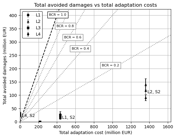
Find adaptations that have a BCR greater than 1
# Find adaptations with BCR greater than 1 under all increase factors
adaptations_with_bcr_greater_than_1 = []
for adapt_id in adapt_ids_output:
    bcr_values = bcr_df.loc[adapt_id]['bcr_mean']
    if all(bcr > 1 for bcr in bcr_values):
        adaptations_with_bcr_greater_than_1.append(adapt_id)
print(f'No-regret: Adaptations with BCR greater than 1 under all increase factors: {adaptations_with_bcr_greater_than_1}')

# Find adaptations with BCR greater than 1 in at least one increase factor but not all 3
adaptations_with_bcr_greater_than_1_some = []
for adapt_id in adapt_ids_output:
    bcr_values = bcr_df.loc[adapt_id]['bcr_mean']
    if any(bcr > 1 for bcr in bcr_values) and not all(bcr > 1 for bcr in bcr_values):
        adaptations_with_bcr_greater_than_1_some.append(adapt_id)
print(f'Adaptations with BCR greater than 1 in at least one increase factor but not all 3: {adaptations_with_bcr_greater_than_1_some}')

# Find adaptations with BCR less than 1 in all increase factors
adaptations_with_bcr_less_than_1 = []
for adapt_id in adapt_ids_output:
    bcr_values = bcr_df.loc[adapt_id]['bcr_mean']
    if all(bcr < 1 for bcr in bcr_values):
        adaptations_with_bcr_less_than_1.append(adapt_id)
print(f'Economically inefficient: Adaptations with BCR less than 1 in all increase factors: {adaptations_with_bcr_less_than_1}')
No-regret: Adaptations with BCR greater than 1 under all increase factors: []
Adaptations with BCR greater than 1 in at least one increase factor but not all 3: []
Economically inefficient: Adaptations with BCR less than 1 in all increase factors: ['baseline', 'l1_trib', 'l2_trib', 'l3_trib', 'l4_trib']
Generate detailed output and maps
# Create a DataFrame with the benefits for each adaptation and increase factor by appending each new Series to the previous one
avoided_damages_df = pd.DataFrame()
for adapt_id in adapt_ids_output:
    for inc_f in increase_factors_bounds.keys():
        new_df = pd.Series(avoided_damages_dict[adapt_id][inc_f], name=(adapt_id, inc_f))
        avoided_damages_df = pd.concat([avoided_damages_df, new_df], axis=1)

avoided_damages_df = avoided_damages_df.T

avoided_damages_df.columns = ['Avoided Direct Y0 [M€/y]', 'Avoided Direct Y100 [M€/y]', 'Avoided Direct Total [M€]', 'Avoided Indirect Tributaries Y0 [M€/y]', 'Avoided Indirect Tributaries Y100 [M€/y]', 'Avoided Indirect Tributaries Total [M€]', 'Avoided Indirect Full Flood Y0 [M€/y]', 'Avoided Indirect Full Flood Y100 [M€/y]', 'Avoided Indirect Full Flood Total [M€]']
avoided_damages_df.index.names = ['Adaptation, Climate Change Increase Factor']

avoided_damages_df.to_csv(data_path / 'output' / 'avoided_damages_df.csv')
avoided_damages_df
| Avoided Direct Y0 [M€/y] | Avoided Direct Y100 [M€/y] | Avoided Direct Total [M€] | Avoided Indirect Tributaries Y0 [M€/y] | Avoided Indirect Tributaries Y100 [M€/y] | Avoided Indirect Tributaries Total [M€] | Avoided Indirect Full Flood Y0 [M€/y] | Avoided Indirect Full Flood Y100 [M€/y] | Avoided Indirect Full Flood Total [M€] | |
|---|---|---|---|---|---|---|---|---|---|
| Adaptation, Climate Change Increase Factor | |||||||||
| (baseline, lower bound) | [0.0, 0.0] | [0.0, 0.0] | [0.0, 0.0] | 0.000 | 0.000 | 0.000 | 0.000 | 0.000 | 0.000 |
| (baseline, mean) | [0.0, 0.0] | [0.0, 0.0] | [0.0, 0.0] | 0.000 | 0.000 | 0.000 | 0.000 | 0.000 | 0.000 |
| (baseline, upper bound) | [0.0, 0.0] | [0.0, 0.0] | [0.0, 0.0] | 0.000 | 0.000 | 0.000 | 0.000 | 0.000 | 0.000 |
| (l1_trib, lower bound) | [0.06795927397899038, 0.19065049132756506] | [0.04049597579089148, 0.12230051654181584] | [5.460906339647906, 15.94745720461816] | 0.046 | 0.034 | 4.200 | 0.002 | 0.001 | 0.174 |
| (l1_trib, mean) | [0.06795927397899038, 0.19065049132756506] | [0.08663090809314511, 0.2572485346597566] | [8.791211640861633, 25.6888413944138] | 0.046 | 0.031 | 3.938 | 0.002 | 0.001 | 0.165 |
| (l1_trib, upper bound) | [0.06795927397899038, 0.19065049132756506] | [0.12862015399657034, 0.38029465429372156] | [11.822255607936285, 34.57107279828983] | 0.046 | 0.028 | 3.729 | 0.002 | 0.001 | 0.157 |
| (l2_trib, lower bound) | [0.19112371926527727, 0.45218484752808075] | [0.12258613834127485, 0.3025187822888218] | [15.985745881166636, 38.72263897122079] | 0.695 | 0.420 | 56.247 | 0.108 | 0.057 | 8.139 |
| (l2_trib, mean) | [0.19112371926527727, 0.45218484752808075] | [0.2318685384791077, 0.5488260285897621] | [23.874426721186182, 56.50262231896508] | 0.695 | 0.605 | 69.576 | 0.108 | 0.051 | 7.704 |
| (l2_trib, upper bound) | [0.19112371926527727, 0.45218484752808075] | [0.3317004586537897, 0.7743284386349978] | [31.080913354999907, 72.78078366295438] | 0.695 | 0.774 | 81.833 | 0.108 | 0.046 | 7.323 |
| (l3_trib, lower bound) | [0.0, 0.0] | [0.0, 0.0] | [0.0, 0.0] | 0.000 | 0.000 | 0.000 | 0.000 | 0.000 | 0.000 |
| (l3_trib, mean) | [0.0, 0.0] | [0.0, 0.0] | [0.0, 0.0] | 0.000 | 0.000 | 0.000 | 0.000 | 0.000 | 0.000 |
| (l3_trib, upper bound) | [0.0, 0.0] | [0.0, 0.0] | [0.0, 0.0] | 0.000 | 0.000 | 0.000 | 0.000 | 0.000 | 0.000 |
| (l4_trib, lower bound) | [0.0, 0.0] | [0.0, 0.0] | [0.0, 0.0] | 0.144 | 0.081 | 11.251 | 0.145 | 0.082 | 11.324 |
| (l4_trib, mean) | [0.0, 0.0] | [0.0, 0.0] | [0.0, 0.0] | 0.144 | 0.117 | 13.818 | 0.145 | 0.117 | 13.887 |
| (l4_trib, upper bound) | [0.0, 0.0] | [0.0, 0.0] | [0.0, 0.0] | 0.144 | 0.149 | 16.168 | 0.145 | 0.150 | 16.234 |
Create geometries for visualisation
od_geoms = get_od_geoms_from_sps(shortest_paths, graph_r0)
od_geoms_plot= gpd.GeoDataFrame(od_geoms)
od_geoms_plot.crs = 'EPSG:3857'
od_geoms_gdf = od_geoms_plot.to_crs('EPSG:4326')
od_geoms_plot.to_file(data_path / 'output' / 'od_geoms_plot.geojson', driver='GeoJSON')
shortest_paths_assets = get_asset_ids_from_sps(shortest_paths, graph_r0)
Prepare geodataframe for plotting
basins_gdf = basins_gdf_0.copy()

# Extract the geometries of the stretches of disrupted rail track
rp_defs = ['L', 'M', 'H']
disrupted_asset_ids = {rp_def: [] for rp_def in rp_defs}
for rp_def in rp_defs:
    for hazard_map, asset_dict in collect_output.items():
        rp = hazard_map.split('_RW_')[-1].split('_')[0]
        if rp != rp_def:
            continue

        overlay_assets = load_baseline_run(hazard_map, interim_data_path, only_overlay=True)
        disrupted_asset_ids[rp_def].extend(overlay_assets.asset.unique())

# Filter out assets that are bridges or tunnels
disrupted_asset_ids_filt = {rp_def: [] for rp_def in rp_defs}
for rp_def, asset_ids in disrupted_asset_ids.items():
    for asset_id in asset_ids:
        if assets.loc[asset_id, 'bridge'] is None and assets.loc[asset_id, 'tunnel'] is None:
            disrupted_asset_ids_filt[rp_def].append(asset_id)

# Prepare gdf for plotting
basins_gdf = basins_gdf_0[basins_gdf_0['HYBAS_ID'].isin(eadD_bl_by_ts_basin_incf['mean'].keys())].copy()
basin_list=basins_gdf.HYBAS_ID.values.tolist()

basins_gdf['Average EAD_D_bl_t0'] = [eadD_bl_by_ts_basin_incf['mean'][basin].values[0].mean() for basin in basin_list]
basins_gdf['Average EAD_D_bl_t100'] = [eadD_bl_by_ts_basin_incf['mean'][basin].values[-1].mean() for basin in basin_list]
basins_gdf['EAD_ID_bl_t0'] = [0.0 if not basin in eadIT_bl_by_ts_basin_incf['mean'].keys() else eadIT_bl_by_ts_basin_incf['mean'][basin].values[0][0] for basin in basin_list]
basins_gdf['EAD_ID_bl_t100'] = [0.0 if not basin in eadIT_bl_by_ts_basin_incf['mean'].keys() else eadIT_bl_by_ts_basin_incf['mean'][basin].values[-1][0] for basin in basin_list]

basins_gdf_reduced = basins_gdf[['HYBAS_ID', 'geometry', 'Average EAD_D_bl_t0', 'Average EAD_D_bl_t100', 'EAD_ID_bl_t0', 'EAD_ID_bl_t100']]
Set plotting style
# import matplotlib.colors as mcolors
import matplotlib.patches as mpatches
import matplotlib as mpl

#Plotting prep
# dic_colors = {'H': '#f03b20', 'M': '#feb24c', 'L': '#ffeda0'} # Yellow, orange, red
dic_colors = {'H': '#9ecae1', 'M': '#3182bd', 'L': '#08519c'} # Blues

main_basin_list = basin_list_full_flood - set(basin_list_tributaries)
assets_4326_clipped = gpd.clip(assets.to_crs(4326), regions_gdf)
basins_gdf_reduced_clipped = gpd.clip(basins_gdf_reduced, regions_gdf)
# Set the font colors
default_mpl_color = miraca_colors['grey_900']
mpl.rcParams['text.color'] = default_mpl_color
mpl.rcParams['axes.labelcolor'] = default_mpl_color
mpl.rcParams['xtick.color'] = default_mpl_color
mpl.rcParams['ytick.color'] = default_mpl_color

fontsize_set = {
    'large': {'title': 42, 'label': 38, 'legend': 20, 'ticks': 28, 'legend_title': 20, 'legend_label': 20, 'suptitle': 16},
    'small': {'title': 24, 'label': 24, 'legend': 18, 'ticks': 16, 'legend_title': 18, 'legend_label': 18, 'suptitle': 12},
    'default_miraca': {'title': 42, 'label': 38, 'legend': 20, 'ticks': 28, 'legend_title': 20, 'legend_label': 20, 'suptitle': 16}
}

mainfont = {'fontname': 'Arial'}
# mainfont = {'fontname': 'Space Grotesk'}
basefont = {'fontname': 'Calibri'}

# Define the size set to use
size_set = fontsize_set['small']  # Change to 'large' or 'small' as needed
Generate plot of damages and losses aggregated by tributaries
# Plot
fig, axs = plt.subplots(2, 2, figsize=(20, 20))
# Direct damages
# Plot for year 0
ax = 0, 0
vmax_dd = math.ceil(max([eadD_bl_by_ts_basin_incf['mean'][basin].values[0].max() for basin in eadD_bl_by_ts_basin_incf['mean']]) / 10.0) * 10
basins_gdf_reduced_clipped.plot(column='Average EAD_D_bl_t0', ax=axs[ax], legend=False, cmap='Reds', vmin=0, vmax=vmax_dd, alpha=0.8)
basins_gdf_reduced_clipped.plot(ax=axs[ax], edgecolor=miraca_colors['grey_200'], facecolor="None", alpha=0.5, linewidth=1)
axs[ax].set_title('Current climate', fontsize=size_set['title'], fontweight='bold', **mainfont)
# Plot for year 100
ax = 0, 1
valid_asset_ids = [asset_id for asset_id in asset_ids if asset_id in assets_4326_clipped.index]
basins_gdf_reduced_clipped.plot(column='Average EAD_D_bl_t100', ax=axs[ax], legend=False, cmap='Reds', vmin=0, vmax=vmax_dd, alpha=0.8)
basins_gdf_reduced_clipped.plot(ax=axs[ax], edgecolor=miraca_colors['grey_200'], facecolor="None", alpha=0.5, linewidth=1)
axs[ax].set_title('Future climate (Future B)', fontsize=size_set['title'], fontweight='bold', **mainfont)
# Add color bar and legend
sm1 = plt.cm.ScalarMappable(cmap='Reds', norm=plt.Normalize(vmin=0, vmax=vmax_dd))
cbar1 = plt.colorbar(sm1, ax=axs[ax])
cbar1.set_label('Direct Expected Annual Damages [Million €/year]', fontsize=size_set['label'], **mainfont)
cbar1.ax.tick_params(labelsize=size_set['ticks'])
rp_letter_equiv = {'H': 'RP10', 'M': 'RP100', 'L': 'RP200'}
legend_elements = [mpatches.Patch(facecolor=dic_colors[rp_def], edgecolor='k', label=rp_letter_equiv[rp_def]) for rp_def in disrupted_asset_ids_filt.keys()]
axs[ax].legend(handles=legend_elements, title='Disrupted Assets', loc='upper left', fontsize=size_set['legend_label'], title_fontsize=size_set['legend_title'])
plt.setp(axs[ax].texts, family='Space Grotesk')

# Indirect losses, tributary basins
# Plot for year 0
ax = 1, 0
vmax_id = np.ceil(max([eadIT_bl_by_ts_basin_incf['mean'][basin].values[0].max() for basin in eadIT_bl_by_ts_basin_incf['mean']]))
basins_gdf_reduced_clipped.plot(column='EAD_ID_bl_t0', ax=axs[ax], legend=False, cmap='Purples', vmin=0, vmax=vmax_id, alpha=0.8)
basins_gdf_reduced_clipped.plot(ax=axs[ax], edgecolor=miraca_colors['grey_200'], facecolor="None", alpha=0.5, linewidth=1)
basins_gdf_reduced_clipped[basins_gdf_reduced_clipped['HYBAS_ID'].isin(main_basin_list)].plot(ax=axs[ax], edgecolor='None', facecolor=miraca_colors['grey_500'], alpha=0.5, linewidth=1, hatch='//')
axs[ax].set_title(' ', fontsize=size_set['title'])
# Plot for year 100
ax = 1, 1
basins_gdf_reduced_clipped.plot(column='EAD_ID_bl_t100', ax=axs[ax], legend=False, cmap='Purples', vmin=0, vmax=1.1*vmax_id, alpha=0.8)
basins_gdf_reduced_clipped.plot(ax=axs[ax], edgecolor=miraca_colors['grey_200'], facecolor="None", alpha=0.5, linewidth=1)
basins_gdf_reduced_clipped[basins_gdf_reduced_clipped['HYBAS_ID'].isin(main_basin_list)].plot(ax=axs[ax], edgecolor='None', facecolor=miraca_colors['grey_500'], alpha=0.5, linewidth=1, hatch='//')
axs[ax].set_title(' ', fontsize=size_set['title'])
# Add color bar
sm2 = plt.cm.ScalarMappable(cmap='Purples', norm=plt.Normalize(vmin=0, vmax=vmax_id))
cbar2 = plt.colorbar(sm2, ax=axs[ax], ticks=[0, 1, 2, 3, 4])
cbar2.set_label('Indirect Expected Annual Losses [Million €/year]', fontsize=size_set['label'], **mainfont)
cbar2.ax.tick_params(labelsize=size_set['ticks'])

# Plot static content
for ax in axs.flat:
    assets_4326_clipped.plot(ax=ax, color=miraca_colors['black'], lw=2)
    for rp_def, asset_ids in disrupted_asset_ids_filt.items():
        valid_asset_ids = [asset_id for asset_id in asset_ids if asset_id in assets_4326_clipped.index]
        assets_4326_clipped.loc[valid_asset_ids].plot(ax=ax, color=dic_colors[rp_def], lw=3)
    regions_gdf.boundary.plot(ax=ax, edgecolor=miraca_colors['blue_900'], linestyle='-', linewidth=0.5)
    ax.set_axis_off()

# Label as A, B, C, D in the bottom right corner with a grey background and black text
for i, ax in enumerate(axs.flat):
    ax.text(0.98, 0.05, f' {chr(65+i)} ', transform=ax.transAxes, fontsize=size_set['title'], fontweight='regular', color='black', ha='center', va='center', bbox=dict(facecolor='lightgrey', edgecolor='black', boxstyle='square,pad=0.2'))
plt.tight_layout()
plt.suptitle('Direct and Indirect Damages and Losses at Year 0 and 100 (Future B) [Baseline]', fontsize=size_set['suptitle'], fontweight='bold', y=1.03, **basefont)
plt.text(0, -0.1, f'Adaptation: No adaptation', ha='center', va='bottom', fontsize=size_set['suptitle'], transform=plt.gca().transAxes, **basefont)

plt.show()
findfont: Font family 'Calibri' not found.
findfont: Font family 'Calibri' not found.
findfont: Font family 'Calibri' not found.
findfont: Font family 'Calibri' not found.
findfont: Font family 'Calibri' not found.
findfont: Font family 'Calibri' not found.
findfont: Font family 'Calibri' not found.
findfont: Font family 'Calibri' not found.
findfont: Font family 'Calibri' not found.
findfont: Font family 'Calibri' not found.
Find the fraction of railways affected
# Save the exposed assets to a GeoJSON file
for rp_def, asset_ids in disrupted_asset_ids_filt.items():
    valid_asset_ids = [asset_id for asset_id in asset_ids if asset_id in assets_4326_clipped.index]
    assets_4326_clipped.loc[valid_asset_ids].to_parquet(data_path / 'output' / 'impacts' / f'exposed_assets_{rp_def}.pq')

output_disruption_summary_path = data_path / 'output' / 'disruption_summary.csv'
calculate_disruption_summary(disrupted_asset_ids_filt, assets_4326_clipped, assets, save_to_csv=True, output_path=output_disruption_summary_path)
Total exposed assets: 73
Total assets: 537
Fraction of disrupted assets: 0.14
Fraction of disrupted asset by length: 0.23
Zooming to the areas with adapted assets
# Plot
fig, axs = plt.subplots(2, 2, figsize=(10, 10))

# Find value max for color bars assuming baseline conditions have higher damages than adapted conditions
baseline_basins_gdf = prep_adapted_basins_gdf(basins_gdf_0, eadD_ad_by_ts_basin_incf, eadIT_ad_by_ts_basin_incf, adapt_id='baseline', inc_f='mean', clipping_gdf=regions_gdf)
vmax_dd = math.ceil(max([baseline_basins_gdf['Average EAD_D_ad_t0'].max(), baseline_basins_gdf['Average EAD_D_ad_t100'].max()]) / 10.0) * 10
vmax_id = np.ceil(max([baseline_basins_gdf['EAD_ID_ad_t0'].max(), baseline_basins_gdf['EAD_ID_ad_t100'].max()]))
adapted_basins_list = find_adapted_basin(eadD_ad_by_ts_basin_incf, eadIT_ad_by_ts_basin_incf, adapt_id='l1_trib')
# xmin, ymin, xmax, ymax = basins_gdf[basins_gdf['HYBAS_ID']==2080430320].total_bounds
xmin, ymin, xmax, ymax = basins_gdf[basins_gdf['HYBAS_ID'].isin(adapted_basins_list)].total_bounds
buffer = 0.05
xmin -= buffer
ymin -= buffer
xmax += buffer
ymax += buffer

# Plot standard elements for all subplots
for ax in axs.flat:
    assets_4326_clipped.plot(ax=ax, color=miraca_colors['black'], markersize=1)
    for rp_def, asset_ids in disrupted_asset_ids_filt.items():
        valid_asset_ids = [asset_id for asset_id in asset_ids if asset_id in assets_4326_clipped.index]
        assets_4326_clipped.loc[valid_asset_ids].plot(ax=ax, color=dic_colors[rp_def], markersize=2, linewidth=3)
    baseline_basins_gdf.plot(ax=ax, edgecolor=miraca_colors['grey_200'], facecolor="None", alpha=0.5, linewidth=1)
    regions_gdf.boundary.plot(ax=ax, edgecolor=miraca_colors['blue_900'], linestyle='-', linewidth=0.5)

    ax.set_axis_off()
    ax.set_xlim(xmin, xmax)
    ax.set_ylim(ymin, ymax)

# Level 1 adaptation
# Plot for year 100
ax = 0, 0
adapt_id = 'l1_trib'
adapted_basins_gdf = prep_adapted_basins_gdf(basins_gdf, eadD_ad_by_ts_basin_incf, eadIT_ad_by_ts_basin_incf, adapt_id=adapt_id, inc_f='mean', clipping_gdf=regions_gdf)
adapted_basins_gdf.plot(column='Average EAD_D_ad_t100', ax=axs[ax], legend=False, cmap='Blues', vmin=0, vmax=vmax_dd, alpha=0.8)
axs[ax].set_title('Level 1 adaptation', fontsize=16, fontweight='bold')
# kevel 1 adaptation is a gdf of the protected area and a filter of the protected assets
gdf_prot_area = gpd.read_file(data_path / 'input' / 'adaptations' /  'l1_tributary.geojson')
assets_adapt=filter_assets_to_adapt(assets_4326_clipped.to_crs(3857), gdf_prot_area.to_crs(3857))
assets_adapt=assets_adapt.to_crs(4326)
gdf_prot_area.plot(ax=axs[ax], edgecolor='black', facecolor=miraca_colors['green_success'], alpha=0.2, linewidth=0.5)
assets_adapt.plot(ax=axs[ax], color='green', lw=4)
assets_adapt.to_file(data_path / 'output' / 'adaptations' / 'l1_tributary_assets.geojson', driver='GeoJSON')

# Level 2 adaptation
# Plot for year 100
ax = 0, 1
adapt_id = 'l2_trib'
adapted_basins_gdf = prep_adapted_basins_gdf(basins_gdf, eadD_ad_by_ts_basin_incf, eadIT_ad_by_ts_basin_incf, adapt_id=adapt_id, inc_f='mean', clipping_gdf=regions_gdf)
adapted_basins_gdf.plot(column='Average EAD_D_ad_t100', ax=axs[ax], legend=False, cmap='Blues', vmin=0, vmax=vmax_dd, alpha=0.8)
axs[ax].set_title('Level 2 adaptation', fontsize=16, fontweight='bold')
# level 2 adaptation is a gdf of the filter of the protected assets
gdf_prot_area = gpd.read_file(data_path / 'input' / 'adaptations' /  'l2_tributary.geojson')
assets_adapt=filter_assets_to_adapt(assets_4326_clipped.to_crs(3857), gdf_prot_area.to_crs(3857))
assets_adapt=assets_adapt.to_crs(4326)
assets_adapt.plot(ax=axs[ax], color='green', lw=4)
assets_adapt.to_file(data_path / 'output' / 'adaptations' / 'l2_tributary_assets.geojson', driver='GeoJSON')

# Level 3 adaptation
# Plot for year 100
ax = 1, 0
adapt_id = 'l3_trib'
adapted_basins_gdf = prep_adapted_basins_gdf(basins_gdf, eadD_ad_by_ts_basin_incf, eadIT_ad_by_ts_basin_incf, adapt_id=adapt_id, inc_f='mean', clipping_gdf=regions_gdf)
adapted_basins_gdf.plot(column='Average EAD_D_ad_t100', ax=axs[ax], legend=False, cmap='Blues', vmin=0, vmax=vmax_dd, alpha=0.8)
axs[ax].set_title('Level 3 adaptation', fontsize=16, fontweight='bold')
# level 3 adaptation is a gdf of new connections between the protected assets
added_links = [(219651487, 111997047)]
for i,osm_id_pair in enumerate(added_links):
        graph_v, _ = add_l3_adaptation(graph_r0, osm_id_pair)
gdf_l3_edges = get_l3_gdf(added_links, graph_v)
gdf_l3_edges.plot(ax=axs[ax], color='green', lw=4)
gdf_l3_edges.to_file(data_path / 'output' / 'adaptations' / 'l3_tributary_edges_b.geojson', driver='GeoJSON')

# Level 4 adaptation
# Plot for year 100
ax = 1, 1
adapt_id = 'l4_trib'
adapted_basins_gdf = prep_adapted_basins_gdf(basins_gdf, eadD_ad_by_ts_basin_incf, eadIT_ad_by_ts_basin_incf, adapt_id=adapt_id, inc_f='mean', clipping_gdf=regions_gdf)
adapted_basins_gdf.plot(column='Average EAD_D_ad_t100', ax=axs[ax], legend=False, cmap='Blues', vmin=0, vmax=vmax_dd, alpha=0.8)
axs[ax].set_title('Level 4 adaptation', fontsize=16, fontweight='bold')
# level 4 adaptation is a gdf with the assets in shortest paths with reduced demand
adapted_route_area = gpd.read_file(data_path / 'input' / 'adaptations' /  'l4_tributary.geojson')
demand_reduction_dict = add_l4_adaptation(graph_r0, shortest_paths, adapted_route_area.to_crs(3857))
assets_in_paths = list(set([asset_id for od, (asset_ids, demand) in get_asset_ids_from_sps(shortest_paths, graph_r0).items() for asset_id in asset_ids if asset_id != '']))
assets_adapt=assets_4326_clipped[assets_4326_clipped['osm_id'].isin(assets_in_paths)]
assets_adapt.plot(ax=axs[ax], color='green', lw=4)
assets_adapt.to_file(data_path / 'output' / 'adaptations' / 'l4_tributary_assets.geojson', driver='GeoJSON')

for ax in axs.flat:
    od_geoms_plot.to_crs(4326).plot(ax=ax, edgecolor=miraca_colors['black'], facecolor="None", markersize=40, linewidth=2)

plt.tight_layout()
plt.suptitle('Direct Damages at Year 100 [Adapted]', fontsize=16,
             fontweight='bold',
             y=1.03)
plt.savefig(data_path / 'output' / 'plots' / 'adaptations_disrupted_assets.png', dpi=300)
plt.show()
Applying adaptation: new connection between assets with osm_id  (219651487, 111997047)
Level 3 adaptation
Applying adaptation: shifted demand for routes:  [('node_682', 'node_684'), ('node_684', 'node_682'), ('node_260', 'node_387'), ('node_387', 'node_260'), ('node_387', 'node_434'), ('node_387', 'node_286'), ('node_434', 'node_387'), ('node_286', 'node_387')]
Level 4 adaptation
Produce processed output tables
# Neat table of adaptations for both case studies with descending BCRs, benefits, and costs
adaptation_table = pd.DataFrame()
dict_tags_names = {'l1': 'L1: flood wall',
                         'l2': 'L2: elevate rail (viaduct)',
                         'l3': 'L3: build new connection',
                         'l4': 'L4: reduce demand',
                         'trib': 'Study Area 2',
                         'rhine': 'Study Area 1',
                         'baseline': 'No adaptation',
                         'upper bound': 'Future C',
                         'lower bound': 'Future A',
                         'mean': 'Future B'}

for adapt_id in adapt_ids_output:
    if adapt_id == 'baseline': continue
    name_components = adapt_id.split('_')
    adaptation_name = dict_tags_names[name_components[0]]
    study_area = dict_tags_names[name_components[1]] if len(name_components) > 1 else 'Unknown'
    for inc_f in increase_factors_bounds.keys():
        bcr_values = bcr_df.loc[adapt_id]['bcr_'+inc_f.split(' ')[0]].mean()
        # npv_values = npv_df.loc[adapt_id]['npv_mean'].mean()
        benefits = benefits_dict[adapt_id][inc_f]['total_avoided_damages_full_period'].mean()
        costs = processed_adaptation_costs[adapt_id]
        # new_row = pd.DataFrame({'Adaptation': [adapt_id], 'BCR': [bcr_values], 'Benefits': [benefits], 'Costs': [costs]})
        new_row = pd.DataFrame({'Adaptation': [adaptation_name], 'Study Area': [study_area], 'BCR': [bcr_values], 'Benefits': [benefits], 'Costs': [costs]})
        adaptation_table = pd.concat([adaptation_table, new_row], ignore_index=True)

# make study area a level for sorting and merge all the rows in a single cell
adaptation_table['Study Area'] = pd.Categorical(adaptation_table['Study Area'], ['Study Area 1', 'Study Area 2', 'Unknown'])
adaptation_table = adaptation_table.sort_values(by=['Study Area', 'BCR'], ascending=[True, False])
# adaptation_table = adaptation_table.sort_values(by='BCR', ascending=False)
adaptation_table.to_csv(data_path / 'output' / 'adaptation_table.csv')
adaptation_table
| Adaptation | Study Area | BCR | Benefits | Costs | |
|---|---|---|---|---|---|
| 5 | L2: elevate rail (viaduct) | Study Area 2 | 0.098 | 141.086 | 1,360.178 |
| 4 | L2: elevate rail (viaduct) | Study Area 2 | 0.086 | 117.468 | 1,360.178 |
| 3 | L2: elevate rail (viaduct) | Study Area 2 | 0.074 | 91.740 | 1,360.178 |
| 2 | L1: flood wall | Study Area 2 | 0.068 | 27.082 | 435.727 |
| 1 | L1: flood wall | Study Area 2 | 0.049 | 21.343 | 435.727 |
| 0 | L1: flood wall | Study Area 2 | 0.029 | 15.079 | 435.727 |
| 6 | L3: build new connection | Study Area 2 | 0.000 | 0.000 | 215.266 |
| 7 | L3: build new connection | Study Area 2 | 0.000 | 0.000 | 215.266 |
| 8 | L3: build new connection | Study Area 2 | 0.000 | 0.000 | 215.266 |
| 9 | L4: reduce demand | Study Area 2 | 0.000 | 22.575 | 0.000 |
| 10 | L4: reduce demand | Study Area 2 | 0.000 | 27.705 | 0.000 |
| 11 | L4: reduce demand | Study Area 2 | 0.000 | 32.402 | 0.000 |
bcr_df_beautified = bcr_df.copy()
bcr_df_beautified['Adaptation'] = bcr_df_beautified.index.map(lambda x: dict_tags_names[x[0].split('_')[0]])
bcr_df_beautified['Study Area'] = bcr_df_beautified.index.map(lambda x: dict_tags_names[x[0].split('_')[1]] if len(x[0].split('_')) > 1 else 'Unknown')
bcr_df_beautified['Future Climate'] = bcr_df_beautified.index.map(lambda x: dict_tags_names[x[1]])
bcr_df_beautified['string_id'] = bcr_df_beautified.index.map(lambda x: x[0] + '_' + x[1])

#add index level to dataframe (study area)
bcr_df_beautified = bcr_df_beautified.reset_index()
bcr_df_beautified.set_index(['Study Area', 'Adaptation', 'Future Climate'], inplace=True)
bcr_df_beautified = bcr_df_beautified.sort_index()

# New formatted columns
bcr_df_beautified['Benefits (M€)'] = bcr_df_beautified['total_avoided_damages'].map(lambda x: f'{x.mean():.0f}') + ' (' + bcr_df_beautified['total_avoided_damages_lower'].map(lambda x: f'{x:.0f}') + ' - ' + bcr_df_beautified['total_avoided_damages_upper'].map(lambda x: f'{x:.0f}') + ')'
bcr_df_beautified['Costs (M€)'] = bcr_df_beautified['total_adaptation_cost'].map(lambda x: f'{x:.0f}')
bcr_df_beautified['BCR avg (range)'] = bcr_df_beautified['bcr'].map(lambda x: f'{x.mean():.2f}') + ' (' + bcr_df_beautified['bcr_lower'].map(lambda x: f'{x:.2f}') + ' - ' + bcr_df_beautified['bcr_upper'].map(lambda x: f'{x:.2f}') + ')'

# Drop unnecessary columns
drop_cols=['total_avoided_damages','total_avoided_damages_lower', 'total_avoided_damages_mean','total_avoided_damages_upper',  'total_adaptation_cost', 'bcr', 'bcr_mean', 'bcr_lower', 'bcr_upper', 'level_0', 'level_1']
bcr_df_beautified.drop(columns=drop_cols, inplace=True)

# move string id to last column
bcr_df_beautified = bcr_df_beautified[['Benefits (M€)', 'Costs (M€)', 'BCR avg (range)', 'string_id']]

bcr_df_beautified
| Benefits (M€) | Costs (M€) | BCR avg (range) | string_id | |||
|---|---|---|---|---|---|---|
| Study Area | Adaptation | Future Climate | ||||
| Study Area 2 | L1: flood wall | Future A | 15 (10 - 20) | 436 | 0.03 (0.02 - 0.05) | l1_trib_lower bound |
| Future B | 21 (13 - 30) | 436 | 0.05 (0.03 - 0.07) | l1_trib_mean | ||
| Future C | 27 (16 - 38) | 436 | 0.06 (0.04 - 0.09) | l1_trib_upper bound | ||
| L2: elevate rail (viaduct) | Future A | 92 (80 - 103) | 1360 | 0.07 (0.06 - 0.08) | l2_trib_lower bound | |
| Future B | 117 (101 - 134) | 1360 | 0.09 (0.07 - 0.10) | l2_trib_mean | ||
| Future C | 141 (120 - 162) | 1360 | 0.10 (0.09 - 0.12) | l2_trib_upper bound | ||
| L3: build new connection | Future A | 0 (0 - 0) | 215 | 0.00 (0.00 - 0.00) | l3_trib_lower bound | |
| Future B | 0 (0 - 0) | 215 | 0.00 (0.00 - 0.00) | l3_trib_mean | ||
| Future C | 0 (0 - 0) | 215 | 0.00 (0.00 - 0.00) | l3_trib_upper bound | ||
| L4: reduce demand | Future A | 23 (23 - 23) | 0 | 0.00 (0.00 - 0.00) | l4_trib_lower bound | |
| Future B | 28 (28 - 28) | 0 | 0.00 (0.00 - 0.00) | l4_trib_mean | ||
| Future C | 32 (32 - 32) | 0 | 0.00 (0.00 - 0.00) | l4_trib_upper bound | ||
| Unknown | No adaptation | Future A | 0 (0 - 0) | 0 | 0.00 (0.00 - 0.00) | baseline_lower bound |
| Future B | 0 (0 - 0) | 0 | 0.00 (0.00 - 0.00) | baseline_mean | ||
| Future C | 0 (0 - 0) | 0 | 0.00 (0.00 - 0.00) | baseline_upper bound |