Railway Flow Visualisation by Country#
This notebook analyses and visualises railway passenger and freight flows for a selected country. It integrates train station and railway infrastructure data, OD (Origin-Destination) matrices, and the railway network to provide insights into the distribution and magnitude of flows through each railway segment. The workflow includes data loading, network construction, OD matrix preparation, capacity estimation, flow assignment, visualisation, and summary statistics. The output includes maps and tables summarizing flows for each railway, with a focus on the selected country.
1. Imports and Configuration#
This section imports all necessary Python libraries and utility functions, and loads the country boundaries dataset. It ensures the spatial data is in the correct coordinate reference system and filters the boundaries to the European region, preparing the context for subsequent railway flow analysis.
base_path = download('https://zenodo.org/records/18428552/files/MIRACA_Transport_Flow_Model.zip?download=1') / 'data'
outpath = Path('~/.miraca').expanduser() / "output"
outpath.mkdir(exist_ok=True, parents=True)

# Load European countries using shared function
europe_countries = load_europe_countries(base_path)
Loaded 54 countries in Europe region
2. Load Data and Prepare OD Matrices#
This section loads the railway network data, including edges, nodes, stations, and OD matrices for both passengers and freight. It prepares the OD data for further analysis by cleaning and formatting the relevant columns.
print('Loading rail data...')
edges_gdf = convert_crs(gpd.read_parquet(base_path / "Infra_BE/belgium_railway_edges.parquet"), 4326)
nodes_gdf = convert_crs(gpd.read_parquet(base_path / "Infra_BE/belgium_railway_nodes.parquet"), 4326)
stations_df = convert_crs(gpd.read_parquet(base_path / "Infra_BE/belgium_railway_stations.parquet"), 4326)
od_flows_pass = pd.read_parquet(base_path / "ODs_BE/belgium_rail_passenger_OD.parquet")
od_flows_freight = pd.read_parquet(base_path / "ODs_BE/belgium_rail_freight_OD.parquet")
print('Data loaded.')

edges_gdf = compute_travel_time_kh(edges_gdf, speed_col='tag_maxspeed')
edge_src = pick_col(edges_gdf, ['from_id'])
edge_dst = pick_col(edges_gdf, ['to_id'])
node_id_col = pick_col(nodes_gdf, ['id'])
station_id_col = pick_col(stations_df, ['id'])


# Prepare OD data
od_pass = od_flows_pass.copy()
od_freight = od_flows_freight.copy()
od_pass['from_node'] = od_pass['origin_node'].astype(str)
od_pass['to_node']   = od_pass['dest_node'].astype(str)
od_pass = od_pass.dropna(subset=['from_node','to_node'])
od_pass['from_node'] = od_pass['from_node'].astype(str)
od_pass['to_node']   = od_pass['to_node'].astype(str)
od_pass['trips']     = pd.to_numeric(od_pass['trips'], errors='coerce').fillna(0.0)
# Drop original node columns to avoid confusion
od_pass = od_pass.drop(columns=['origin_node', 'dest_node'], errors='ignore')
od_pass = od_pass[od_pass['trips'] > 0]

od_freight['from_node'] = od_freight['from_id'].astype(str)
od_freight['to_node']   = od_freight['to_id'].astype(str)
od_freight = od_freight.dropna(subset=['from_node','to_node'])
od_freight['from_node'] = od_freight['from_node'].astype(str)
od_freight['to_node']   = od_freight['to_node'].astype(str)
od_freight['ths_tons']     = pd.to_numeric(od_freight['value'], errors='coerce').fillna(0.0)
od_freight = od_freight[od_freight['ths_tons'] > 0]
Loading rail data...
Data loaded.
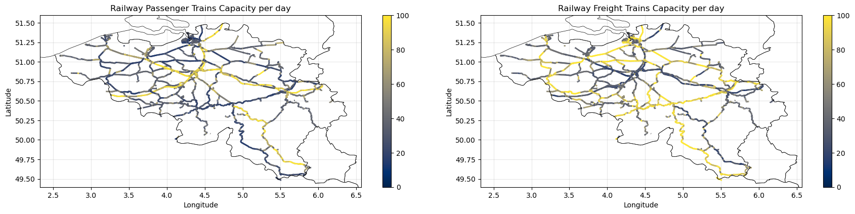
3. Compute and Visualise Capacities#
This section estimates per-edge capacities for both passenger and freight trains based on operational assumptions. It visualises the number of trains per edge and sets up the network for flow assignment.
edges_gdf = edges_gdf.copy()
edges_gdf['edge_id'] = np.arange(len(edges_gdf), dtype=int)


network_df = pd.DataFrame({
    'from_node': edges_gdf[edge_src].astype(str).values,
    'to_node':   edges_gdf[edge_dst].astype(str).values,
    'edge_id':   edges_gdf['edge_id'].values,
    'travel_time': pd.to_numeric(edges_gdf['travel_time'], errors='coerce').fillna(1.0).astype(float).values,
    'CORRIDORS': edges_gdf['CORRIDORS'].values
})

network_df['trips'] = 0.0
network_df['ths_tons'] = 0.0
rng = np.random.default_rng(42)
train_draw_tons = np.maximum(rng.normal(700.0/1000, 35.0/1000, size=len(edges_gdf)), 0.0)
occ_draw_tons   = np.clip(rng.normal(0.90, 0.09, size=len(edges_gdf)), 0.0, 1.0)
eff_tons   = train_draw_tons * occ_draw_tons
cap_tons = compute_edge_capacity(edges_gdf, tt_col='travel_time', train_tons=eff_tons, mode='Freight')
cap_arr_tons = np.asarray(cap_tons, dtype=float)
cap_arr_tons = np.where(np.isfinite(cap_arr_tons), cap_arr_tons, 0.0)
network_df['capacity_ths_tons'] = cap_arr_tons

train_draw_pass = np.maximum(rng.normal(300.0, 15.0, size=len(edges_gdf)), 0.0)
occ_draw_pass   = np.clip(rng.normal(0.50, 0.05, size=len(edges_gdf)), 0.0, 1.0)
eff_pass   = train_draw_pass * occ_draw_pass
cap_pass = compute_edge_capacity(edges_gdf, tt_col='travel_time', train_tons=eff_pass, mode='Passenger')
cap_arr_pass = np.asarray(cap_pass, dtype=float)
cap_arr_pass = np.where(np.isfinite(cap_arr_pass), cap_arr_pass, 0.0)
network_df['capacity_pass'] = cap_arr_pass

# Plot the number of trains per edge based on cap_arr_pass / eff_pass and cap_arr_tons / eff_tons
num_trains_pass = np.where(eff_pass > 0, cap_arr_pass / eff_pass, 0)
num_trains_freight = np.where(eff_tons > 0, cap_arr_tons / eff_tons, 0)

fig, ax = plt.subplots(1, 2, figsize=(18, 4))

edges_gdf_copy = edges_gdf.copy()
edges_gdf_copy['num_trains_pass'] = num_trains_pass/300
edges_gdf_copy['num_trains_freight'] = num_trains_freight/300

# Get Belgium geometry and bounds using helper function
xlim, ylim = get_country_bounds(europe_countries, 'belgium')

# Plot Passenger Trains
edges_gdf_copy.plot(ax=ax[0], column='num_trains_pass', cmap='cividis', linewidth=2, legend=True, vmin=0, vmax=100)
europe_countries.boundary.plot(ax=ax[0], color='black', linewidth=0.5)
ax[0].set_title('Railway Passenger Trains Capacity per day')
ax[0].set_xlabel('Longitude')
ax[0].set_ylabel('Latitude')
ax[0].set_xlim(xlim)
ax[0].set_ylim(ylim)
ax[0].grid(True, alpha=0.3)

# Plot Freight Trains
edges_gdf_copy.plot(ax=ax[1], column='num_trains_freight', cmap='cividis', linewidth=2, legend=True, vmin=0, vmax=100)
europe_countries.boundary.plot(ax=ax[1], color='black', linewidth=0.5)
ax[1].set_title('Railway Freight Trains Capacity per day')
ax[1].set_xlabel('Longitude')
ax[1].set_ylabel('Latitude')
ax[1].set_xlim(xlim)
ax[1].set_ylim(ylim)
ax[1].grid(True, alpha=0.3)

plt.tight_layout()
plt.show()
4. Create Network#
This section builds the railway network graph, filters edges by capacity, and prepares the network for flow assignment and further analysis.
thr_capacity = 1
# Filter out edges with capacity below threshold
network_df_filtered = network_df[(network_df['capacity_ths_tons'] >= thr_capacity) & (network_df['capacity_pass'] >= thr_capacity)].copy()
edges_gdf_copy = edges_gdf[edges_gdf['edge_id'].isin(network_df_filtered['edge_id'])].copy()
edges_gdf_copy = edges_gdf_copy.merge(
    network_df_filtered[['edge_id', 'capacity_ths_tons', 'capacity_pass']],
    on='edge_id', how='left'
    )

base_graph = ig.Graph.TupleList(
    network_df_filtered[['from_node', 'to_node', 'edge_id', 'travel_time']].itertuples(index=False, name=None),
    edge_attrs=['edge_id', 'travel_time'],
    directed=False
)

print(f"Network: {base_graph.vcount()} nodes, {base_graph.ecount()} edges in igraph object.")

# total capacities
total_cap_freight = network_df_filtered['capacity_ths_tons'].sum()
total_cap_passenger = network_df_filtered['capacity_pass'].sum()
print(f"Total Freight Capacity (ths tons): {total_cap_freight:,.2f}")
print(f"Total Passenger Capacity: {total_cap_passenger:,.2f}")
Network: 26196 nodes, 30741 edges in igraph object.
Total Freight Capacity (ths tons): 343,659,613.69
Total Passenger Capacity: 67,087,462,445.50
5. Assign Flows to the Network#
This section assigns passenger and freight flows to the railway network using a capacity-constrained allocation algorithm. It aggregates the assigned flows per edge, and merges the results into the network DataFrame.
# Prepare OD flows for allocation
flow_ods_pass = (od_pass[['from_node', 'to_node', 'trips']].groupby(['from_node', 'to_node'], as_index=False)['trips'].sum())
flow_ods_freight = (od_freight[['from_node', 'to_node', 'ths_tons']].groupby(['from_node', 'to_node'], as_index=False)['ths_tons'].sum())

# Run capacity-constrained allocation for passenger trains
capacity_ods_pass, unassigned_paths_pass, filtered_network_df, progress_df = od_flow_allocation_capacity_constrained(
    flow_ods=flow_ods_pass,
    network_dataframe=network_df_filtered,
    flow_column='trips',
    cost_column='travel_time',
    path_id_column='edge_id',
    attribute_list=None,
    origin_id_column='from_node',
    destination_id_column='to_node',
    network_capacity_column='capacity_pass',
    directed=False,
    simple=False,
    store_edge_path=True,
    graph_base=base_graph,
    track_progress=True,
    early_stop_share=0.95
)

# Run capacity-constrained allocation for freiht trains
capacity_ods_freight, unassigned_paths_freight, filtered_network_df, progress_df = od_flow_allocation_capacity_constrained(
    flow_ods=flow_ods_freight,
    network_dataframe=network_df_filtered,
    flow_column='ths_tons',
    cost_column='travel_time',
    path_id_column='edge_id',
    attribute_list=None,
    origin_id_column='from_node',
    destination_id_column='to_node',
    network_capacity_column='capacity_ths_tons',
    directed=False,
    simple=False,
    store_edge_path=True,
    graph_base=base_graph,
    track_progress=True,
    early_stop_share=0.95
)

# Aggregate assigned flows per edge
if isinstance(capacity_ods_pass, list):
    assigned_passenger_df = pd.concat(capacity_ods_pass, ignore_index=True)
else:
    assigned_passenger_df = capacity_ods_pass

if isinstance(capacity_ods_freight, list):
    assigned_freight_df = pd.concat(capacity_ods_freight, ignore_index=True)
else:
    assigned_freight_df = capacity_ods_freight

# Get total assigned trips per edge
assigned_passenger_on_edges = get_flow_on_edges(assigned_passenger_df, 'edge_id', 'edge_path', 'trips')
assigned_freight_on_edges = get_flow_on_edges(assigned_freight_df, 'edge_id', 'edge_path', 'ths_tons')

# Merge back into filtered_network_df
filtered_network_df = filtered_network_df.merge(
    assigned_passenger_on_edges.rename(columns={'trips': 'assigned_passenger_trips'}),
    on='edge_id', how='left'
)
filtered_network_df = filtered_network_df.merge(
    assigned_freight_on_edges.rename(columns={'ths_tons': 'assigned_ths_tons'}),
    on='edge_id', how='left'
)

# Fill NaN with 0 for assigned flows
filtered_network_df['assigned_passenger_trips'] = filtered_network_df['assigned_passenger_trips'].fillna(0.0)
filtered_network_df['assigned_ths_tons'] = filtered_network_df['assigned_ths_tons'].fillna(0.0)

# Ensure filtered_network_df has geometry
filtered_network_df = filtered_network_df.merge(
    edges_gdf[['edge_id', 'geometry']],
    on='edge_id',
    how='left'
)
[progress] iter=0 assigned_iter=100673230.000 cum=100673230.000 (0.9021) remaining=10924472.000 overcap_edges=0 next_flows=0
[progress] iter=0 assigned_iter=31209.418 cum=31209.418 (0.9999) remaining=4.067 overcap_edges=0 next_flows=0
Early stop triggered at share 1.000 (threshold 0.950).
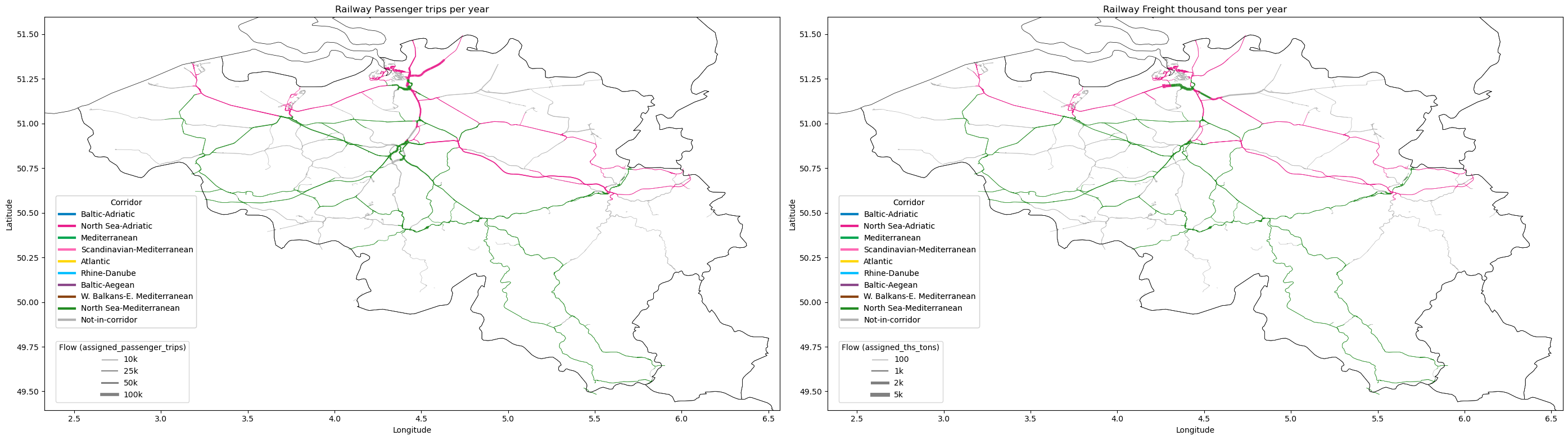
7. Create Flow Visualisation#
This section visualises the assigned passenger and freight flows on the railway network using maps, where line thickness and color represent flow magnitude and corridor, respectively. The maps are zoomed to the selected country and saved as images.
# Set the selected country
SELECTED_COUNTRY = "Belgium"

# Create figure
fig, ax = plt.subplots(1, 2, figsize=(28, 20))

plot_edges_by_flow_thickness(
    ax[0],filtered_network_df, flow_col='assigned_passenger_trips', corridors_col='CORRIDORS',
    lw_min=0.5, lw_max=5, scale='linear', scale_div=100, legend_ticks=[10000,25000,50000,100000]
 )
europe_countries.boundary.plot(ax=ax[0], color='black', linewidth=0.5)
ax[0].set_title('Railway Passenger trips per year')
ax[0].set_xlabel('Longitude')
ax[0].set_ylabel('Latitude')
ax[0].set_xlim(xlim)
ax[0].set_ylim(ylim)


plot_edges_by_flow_thickness(
    ax[1],filtered_network_df, flow_col='assigned_ths_tons', corridors_col='CORRIDORS',
    lw_min=0.5, lw_max=5, scale='linear', scale_div=5, legend_ticks=[100,1000,2500,5000]
 )
europe_countries.boundary.plot(ax=ax[1], color='black', linewidth=0.5)
ax[1].set_title('Railway Freight thousand tons per year')
ax[1].set_xlabel('Longitude')
ax[1].set_ylabel('Latitude')
ax[1].set_xlim(xlim)
ax[1].set_ylim(ylim)

plt.savefig(outpath / f'rail_network_{SELECTED_COUNTRY.replace(" ", "_")}.png', dpi=300, bbox_inches='tight')

plt.tight_layout()
plt.show()
5. Summary Statistics#
This section provides summary statistics for the selected country’s rail infrastructure and flows. It reports the total freight and passenger flows, and net flows, offering a concise overview of the country’s railway activity.
# Print summaries using helper function
print_capacity_flow_summary(od_pass, capacity_ods_pass, 'trips', 'PASSENGER')
print_capacity_flow_summary(od_freight, capacity_ods_freight, 'ths_tons', 'FREIGHT', 'ths tons')
print("=" * 80)
================================================================================
PASSENGER FLOW SUMMARY
================================================================================
Total OD pairs: 39,650
Total trips: 111,597,702
Max edge flow (passenger): 1,026,446
Mean edge flow (passenger): 2,622

================================================================================
FREIGHT FLOW SUMMARY
================================================================================
Total OD pairs: 15,382
Total ths_tons: 31,213 ths tons
Max edge flow (freight): 3,639 ths tons
Mean edge flow (freight): 3 ths tons

================================================================================