Climate risk assessment for transport infrastructure#
In this notebook, we will perform a damage and risk assessment for transport infrastructure, specifically focusing on roads. The assessment is based on combining hazard data (e.g., flood depths) with vulnerability curves to estimate the potential damage to infrastructure.
We will follow the steps outlined below to conduct the assessment:
Loading the necessary packages:
We will import the Python libraries required for data handling, analysis, and visualization.Loading the data:
The infrastructure data (e.g., roads) and hazard data (e.g., flood depths) will be loaded into the notebook.Preparing the data:
The infrastructure and hazard data will be processed and data gaps can be filled, if required.Performing the damage assessment:
We will apply vulnerability curves to estimate the potential damage based on the intensity of the hazard.Visualising the results:
Finally, we will visualise the estimated damage using graphs and maps to illustrate the impact on transport infrastructure.
1. Loading the required Packages#
To perform the assessment, we are going to make use of several python packages.
In case you run this in Google Colab, you will have to install the packages below (remove the hashtag in front of them).
In this step, we will import all the required Python libraries for data manipulation, spatial analysis, and visualization.
Specify the country of interest#
Before we continue, we should specify the country for which we want to assess the damage. We use the ISO3 code for the country to download the OpenStreetMap data.
country_full_name = 'Belgium'
country_iso3 = 'BEL'
2. Loading the Data#
In this step, we will load four key datasets:
Infrastructure data:
This dataset contains information on the location and type of transport infrastructure (e.g., roads). Each asset may have attributes such as type, length, and replacement cost.Hazard data:
This dataset includes information on the hazard affecting the infrastructure (e.g., flood depth at various locations).Vulnerability curves:
Vulnerability curves define how the infrastructure’s damage increases with the intensity of the hazard. For example, flood depth-damage curves specify how much damage occurs for different flood depths.Maximum damage values:
This dataset contains the maximum possible damage (in monetary terms) that can be incurred by individual infrastructure assets. This is crucial for calculating total damage based on the vulnerability curves.
Infrastructure Data#
We will perform this example analysis for Belgium. To start the analysis, we first download the OpenStreetMap data from GeoFabrik. In case of locally available data, one can load the shapefiles with Geopandas, with gpd.read_file(), as we show in the second cell within this section.
infrastructure_path = download.get_country_geofabrik(country_iso3)
Now we load the data and read only the road data.
%%time
features = gpd.read_file(infrastructure_path, layer="lines")
features = features[features["highway"].values != None]
CPU times: user 36.4 s, sys: 30.8 s, total: 1min 7s
Wall time: 5min 20s
[!NOTE]
Depending on the size of the country, loading the critical infrastructure might take some minutes. For this example, the run time takes approximately 2 minutes, depending on the local machine.
sub_types = ['motorway', 'motorway_link', 'trunk', 'trunk_link',
                            'primary', 'primary_link', 'secondary', 'secondary_link', 'tertiary',
                            'tertiary_link', 'residential', 'road', 'unclassified','track']
features = features[features['highway'].isin(sub_types)].reset_index(drop=True)
In OpenStreetMap, these are many subtypes that can be considered. To simplify the analysis, we combine some subtypes.
features = features.replace({'highway' : { 'motorway_link' : 'motorway',
                         'trunk_link' : 'trunk',
                         'primary_link' : 'primary' ,
                        'secondary_link' : 'secondary',
                         'tertiary_link' : 'tertiary',
                         'primary_link' : 'primary',
                         'residential' : 'other' ,
                        'road' : 'other',
                         'unclassified' : 'other',
                         'track' : 'other',
                              }})
Now define a new set of sub_types, to be used in the remainder of this analysis:
sub_types = ['motorway', 'trunk','primary', 'secondary', 'tertiary', 'other']
Hazard Data#
For this example, we make use of the flood data provided by CDRI.
We use a flood hazard map with a probability of ocurrence of 1 in 100 years return period to showcase the approach.
hazard_map = xr.open_dataset("https://hazards-data.unepgrid.ch/global_pc_h100glob.tif", engine="rasterio")
hazard_map
<xarray.Dataset> Size: 747GB
Dimensions:      (band: 1, x: 432000, y: 216000)
Coordinates:
  * band         (band) int64 8B 1
  * x            (x) float64 3MB -180.0 -180.0 -180.0 ... 180.0 180.0 180.0
  * y            (y) float64 2MB 90.0 90.0 90.0 90.0 ... -90.0 -90.0 -90.0 -90.0
    spatial_ref  int64 8B ...
Data variables:
band_data (band, y, x) float64 746GB ...Maximum damages#
One of the most difficult parts of the assessment is to define the maximum reconstruction cost of particular assets. Here we provide a baseline set of values, but these should be updated through national consultations.
maxdam_dict = {'trunk':2000,
               'motorway' : 2000,
                'primary':2000,
                'secondary':1300,
                'tertiary':700,
                'other':300 }
To be used in our damage assessment, we convert this to a Pandas DataFrame
maxdam = pd.DataFrame.from_dict(maxdam_dict,orient='index').reset_index()
maxdam.columns = ['object_type','damage']
And check if any of the objects are missing from the dataframe.
missing = set(sub_types) - set(maxdam.object_type)

if len(missing) > 0:
    print(f"Missing object types in maxdam: \033[1m{', '.join(missing)}\033[0m. Please add them before you continue.")
Vulnerability data#
Similarly to the maximum damages, specifying the vulnerability curves is complex. We generally have limited information about the quality of the assets, its level of deteriation and other asset-level characteristics. The study by Nirandjan et al. (2024) provides us with a baseline set of fragility and vulnerability curves that one can use. In the following cell, we load that data.
vulnerability_path = "https://zenodo.org/records/10203846/files/Table_D2_Multi-Hazard_Fragility_and_Vulnerability_Curves_V1.0.0.xlsx?download=1"
vul_df = pd.read_excel(vulnerability_path,sheet_name='F_Vuln_Depth')
By filtering the vulnerability curves to those relevant for river flooding, F_Vuln_Depth we can explore all the available options:
with pd.option_context('display.max_rows', None, 'display.max_colwidth', None):
  display(vul_df.iloc[:2,:].T)
| 0 | 1 | |
|---|---|---|
| ID number | Infrastructure description | Additional characteristics |
| F1.1 | plant | Small power plants, capacity <100 MW |
| F1.2 | plant | Medium power plants, capacity 100-500 MW |
| F1.3 | plant | Large power plants, >500 MW |
| F1.4 | plant | thermal plant |
| F1.5 | plant | wind turbine |
| F1.6 | plant | wind turbine |
| F1.7 | plant | wind turbine |
| F2.1 | substation | Low Voltage Substation |
| F2.2 | substation | Medium Voltage Substation |
| F2.3 | substation | High Voltage Substation |
| F5.1 | cable | Distribution circuits buried crossings |
| F6.1 | Power (minor) line | Distribution circuits (non-crossings) |
| F6.2 | cable | Distribution circuits elevated crossings |
| F6.3 | Energy system | Generalized curve for energy assets in diked areas |
| F7.1 | Roads | NaN |
| F7.2 | Roads | NaN |
| F7.2a (lower boundary) | Roads | NaN |
| F7.2b (upper boundary) | Roads | NaN |
| F7.3 | Roads | NaN |
| F7.4 | Roads | Motorways and trunk roads - sophisticated accessories - low flow |
| F7.5 | Roads | Motorways and trunk roads - sophisticated accessories - high flow |
| F7.6 | Roads | Motorways and trunk roads - without sophisticated accessories - low flow |
| F7.7 | Roads | Motorways and trunk roads - without sophisticated accessories - high flow |
| F7.8 | Roads | Other roads - low flow |
| F7.9 | Roads | Other roads - high flow |
| F7.10 | Roads | NaN |
| F7.11 | Roads | NaN |
| F7.12 | Roads | NaN |
| F7.13 | Roads | NaN |
| F8.1 | Railways | Double-tracked railway |
| F8.2 | Railways | Double-tracked railway |
| F8.3 | Railways | NaN |
| F8.4 | Railways | NaN |
| F8.5 | Railways | NaN |
| F8.6 | Railways | NaN |
| F8.6a (lower boundary) | Railways | NaN |
| F8.6b (upper boundary) | Railways | NaN |
| F8.7 | Railways | NaN |
| F8.8 | Railways | Railway station |
| F9.1 | Airports | NaN |
| F9.2 | Airports | NaN |
| F9.3 | Airports | NaN |
| F10.1 | Telecommunication | Communication tower |
| F12.1 | Telecommunication | Communication system |
| F13.1 | water storage tanks | Water storage tanks at grade concrete |
| F13.2 | water storage tanks | Water storage tanks at grade steel |
| F13.3 | water storage tanks | Water storage tanks at grade wood |
| F13.4 | water storage tanks | Water storage tanks elevated |
| F13.5 | water storage tanks | Water storage tanks below grade |
| F14.1 | Water treatment plants | Small water treatment plants open/gravity - average flood design |
| F14.2 | Water treatment plants | Medium water treatment plants open/gravity - average flood design |
| F14.3 | Water treatment plants | Large water treatment plants open/gravity - average flood design |
| F14.4 | Water treatment plants | small/medium/large water treatment plants open/gravity - above average flood design |
| F14.5 | Water treatment plants | small/medium/large water treatment plants open/gravity - below average flood design |
| F14.6 | Water treatment plants | Small water treatment plants closed/pressure |
| F14.7 | Water treatment plants | Medium water treatment plants closed/pressure |
| F14.8 | Water treatment plants | Large water treatment plants closed/pressure |
| F14.9 | Water treatment plants | small/medium/large water treatment plants closed/pressure - above average flood design |
| F14.10 | Water treatment plants | small/medium/large water treatment plants closed/pressure - below average flood design |
| F15.1 | Water well | Wells |
| F16.1 | Transmission and distribution pipelines | Exposed transmission pipeline crossing |
| F16.2 | Transmission and distribution pipelines | Buried transmission pipeline crossing |
| F16.3 | Transmission and distribution pipelines | Pipelines (non-crossing) |
| F17.1 | Others | Pumping plants (small) below grade |
| F17.2 | Others | Pumping plants (medium/large) below grade |
| F17.3 | Others | Pumping plants (small) above grade |
| F17.4 | Others | Pumping plants (medium/large) above grade |
| F17.5 | Others | Pumping plants |
| F17.6 | Others | Control vaults and stations |
| F18.1 | Wastewater treatment plant | Small wastewater treatment plants |
| F18.2 | Wastewater treatment plant | Medium wastewater treatment plants |
| F18.3 | Wastewater treatment plant | Large wastewater treatment plants |
| F18.4 | Wastewater treatment plant | Small, medium, large Wastewater treatment plants - above average flood design |
| F18.5 | Wastewater treatment plant | Small, medium, large Wastewater treatment plants- below average flood design |
| F18.6 | Wastewater treatment plant | NaN |
| F19.1 | Transmission and distribution pipelines | Sewers & Interceptors: Exposed collector river crossings |
| F19.2 | Transmission and distribution pipelines | Sewers & Interceptors: Buried collector river crossings |
| F19.3 | Transmission and distribution pipelines | Sewers & Interceptors: Pipes (non-crossings) |
| F20.1 | Others | Control vaults and control stations |
| F20.2 | Others | Lift stations: lift station (small), wet well/dry well |
| F20.3 | Others | Lift stations: lift station (medium large), wet well/dry well |
| F20.4 | Others | Lift stations: lift station (small), submersible |
| F20.5 | Others | Lift stations: lift station (medium large), submersible |
| F21.1 | Education & Health | Generalized curve for commercial buildings, which also includes schools and hospitals |
| F21.2 | Education & Health | Generalized curve for commercial buildings, which also includes schools and hospitals |
| F21.3 | Education & Health | Generalized curve for commercial buildings, which also includes schools and hospitals |
| F21.3a (lower boundary) | Education & Health | Generalized curve for commercial buildings, which also includes schools and hospitals |
| F21.3b (upper boundary) | Education & Health | Generalized curve for commercial buildings, which also includes schools and hospitals |
| F21.4 | Education & Health | Generalized curve for commercial buildings, which also includes schools and hospitals |
| F21.4a (lower boundary) | Education & Health | Generalized curve for commercial buildings, which also includes schools and hospitals |
| F21.4b (upper boundary) | Education & Health | Generalized curve for commercial buildings, which also includes schools and hospitals |
| F21.5 | Education & Health | Generalized curve for commercial buildings, which also includes schools and hospitals |
| F21.5a (lower boundary) | Education & Health | Generalized curve for commercial buildings, which also includes schools and hospitals |
| F21.5b (upper boundary) | Education & Health | Generalized curve for commercial buildings, which also includes schools and hospitals |
| F21.6 | Education & Health | Generalized curve for commercial buildings, which also includes schools and hospitals |
| F21.7 | School buildings | Generalized curve for companies (incl. government) |
| F21.8 | Health & education | Generalized curve for offices in diked areas |
| F21.9 | Education & Health | Generalized function for industry |
| F21.10 | School buildings | Generalized curve for buildings |
| F21.11 | School buildings | NaN |
| F21.12 | Health buildings | NaN |
| F21.13 | Education buildings | NaN |
And select a curve to use for each different subtype we are analysing.
sub_types
['motorway', 'trunk', 'primary', 'secondary', 'tertiary', 'other']
selected_curves = dict(zip(sub_types,['F7.5','F7.5','F7.5','F7.7','F7.7','F7.9']))
The next step is to extract the curves from the database, and prepare them for proper usage into our analysis.
We start by selecting the curve IDs from the larger pandas DataFrame vul_df:
damage_curves = vul_df[['ID number']+list(selected_curves.values())]
damage_curves = damage_curves.iloc[4:125,:]
Then for convenience, we rename the index name to the hazard intensity we are considering.
damage_curves.set_index('ID number',inplace=True)
damage_curves.index = damage_curves.index.rename('Depth')
And make sure that our damage values are in floating numbers.
damage_curves = damage_curves.astype(np.float32)
And ensure that the columns of the curves link back to the different asset types we are considering:
damage_curves.columns = sub_types
There could be some NaN values at the tail of some of the curves. To make sure the code works, we fill up the NaN values with the last value of each of the curves.
damage_curves = damage_curves.ffill()
#damage_curves = damage_curves.fillna(method='ffill')
Finally, make sure we set the index of the damage curves (the inundation depth) in the same metric as the hazard data (e.g. meters or centimeters).
damage_curves.index = damage_curves.index*100
Ancilliary data for processing#
world = gpd.read_file("https://github.com/nvkelso/natural-earth-vector/raw/master/10m_cultural/ne_10m_admin_0_countries.shp")
world_plot = world.to_crs(3857)
admin1 = gpd.read_file("https://github.com/nvkelso/natural-earth-vector/raw/master/10m_cultural/ne_10m_admin_1_states_provinces.shp")
3. Preparing the Data#
Change the column name of the object data, to ensure we can use the same functions across different infrastructure assets
features = features.rename(columns = {'highway' : 'object_type'})
Clip the hazard data to the country of interest. For Belgim, the country_iso3 is BEL
country_bounds = world.loc[world.ADM0_ISO == country_iso3].bounds
country_geom = world.loc[world.ADM0_ISO == country_iso3].geometry
hazard_country = hazard_map.rio.clip_box(minx=country_bounds.minx.values[0],
                     miny=country_bounds.miny.values[0],
                     maxx=country_bounds.maxx.values[0],
                     maxy=country_bounds.maxy.values[0]
                    )
hazard_country = hazard_country.rio.set_crs(4326)
4. Performing an Exposure Assessment#
We will use the DamageScanner approach. This is a fully optimised damage calculation method, that can capture a wide range of inputs to perform a damage assessment. It also allows to only assess the potential exposure.
exposure_results = DamageScanner(hazard_country, features, damage_curves, maxdam).exposure()
Overlay raster with vector: 100%|██████████| 40/40 [02:03<00:00,  3.08s/it]
convert coverage to meters: 100%|██████████| 720488/720488 [00:17<00:00, 40972.56it/s]
5. Performing a Vulnerability Assessment#
In some cases, the cost information is unavailable, or one wants to explore only the exposure and vulnerability. To do so, we simply run the DamageScanner, by setting the maximum costs to 1.
vulnerability_maxdam = maxdam.copy()
vulnerability_maxdam.loc[:,'damage'] = maxdam['damage']/maxdam['damage']
%%time
vulnerability_results = DamageScanner(hazard_country, features, damage_curves, vulnerability_maxdam).calculate()
Overlay raster with vector: 100%|██████████| 40/40 [02:00<00:00,  3.00s/it]
convert coverage to meters: 100%|██████████| 720488/720488 [00:18<00:00, 39709.88it/s]
Calculating damage: 100%|██████████| 720488/720488 [00:24<00:00, 29436.87it/s]
CPU times: user 2min 57s, sys: 6.81 s, total: 3min 4s
Wall time: 3min 6s
6. Performing the Damage Assessment#
In case we do have cost values, we can fully assess the damages. The function DamageScanner uses four main inputs to assess t
%%time
damage_results = DamageScanner(hazard_country, features, damage_curves, maxdam).calculate()
Overlay raster with vector: 100%|██████████| 40/40 [02:00<00:00,  3.00s/it]
convert coverage to meters: 100%|██████████| 720488/720488 [00:18<00:00, 38031.58it/s]
Calculating damage: 100%|██████████| 720488/720488 [00:24<00:00, 28832.17it/s]
CPU times: user 2min 57s, sys: 6.57 s, total: 3min 4s
Wall time: 3min 6s
7. Save the Results#
For further analysis, we can save the results in their full detail, or save summary estimates per subnational unit. We show how to do this using the damage results.
hazard = 'river_flood'
return_period = '1_100'
damage_results.to_file(f'Road_Damage_{country_full_name}_{hazard}_{return_period}.gpkg')
admin1_country = admin1.loc[admin1.sov_a3 == country_iso3]
damage_results = damage_results.sjoin(admin1_country[['adm1_code','name','geometry']])
admin1_damage = admin1_country.merge(damage_results[['name_right','damage']].groupby('name_right').sum(),
                                     left_on='name',
                                     right_on='name_right',
                                     how='outer')[['name','adm1_code','geometry','damage']]
admin1_damage.head()
| name | adm1_code | geometry | damage | |
|---|---|---|---|---|
| 0 | Antwerp | BEL-3480 | POLYGON ((4.76418 51.49624, 4.77865 51.49536, ... | 1.135872e+08 |
| 1 | Brussels | BEL-3474 | POLYGON ((4.47975 50.79542, 4.39843 50.76779, ... | 1.018201e+07 |
| 2 | East Flanders | BEL-3478 | POLYGON ((3.3988 51.2447, 3.42194 51.23798, 3.... | 2.312582e+08 |
| 3 | Flemish Brabant | BEL-3475 | POLYGON ((4.09974 50.70712, 4.07271 50.71291, ... | 3.077080e+07 |
| 4 | Hainaut | BEL-2 | MULTIPOLYGON (((2.88688 50.69665, 2.87128 50.6... | 4.586031e+07 |
admin1_damage.to_file(f'Admin1_Road_Damage_{country_full_name}_{hazard}_{return_period}.gpkg')
8. Visualising the Results#
The results of the damage assessment can be visualised using charts and maps. This will provide a clear representation of which infrastructure is most affected by the hazard and the expected damage levels.
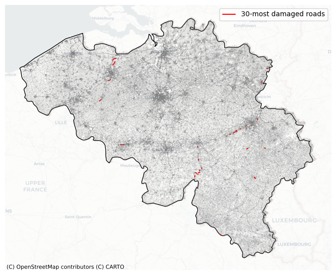
Find the locations of the thirty most damaged roads.
fig, ax = plt.subplots(1,1,figsize=(10, 7))

damage_results.to_crs(3857).sort_values('damage',ascending=False).head(30).plot(ax=ax,color='Red', label="30-most damaged roads")
features.to_crs(3857).plot(ax=ax,facecolor="none",edgecolor='grey',alpha=0.5,zorder=2,lw=0.2)
world_plot.loc[world.SOV_A3 == country_iso3].plot(ax=ax,facecolor="none",edgecolor='black')
cx.add_basemap(ax, source=cx.providers.CartoDB.Positron,alpha=0.5)
ax.set_axis_off()
ax.legend()
<matplotlib.legend.Legend at 0x328cdb390>
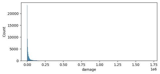
Plot map with damages and the distribution#
To visualise the damages on the map and the histogram for all roads in Belgium, we first filter the database to exclude those transects that are not exposed to river flooding
damage_results = damage_results[damage_results["damage"] != 0]
fig, ax = plt.subplots(1,1,figsize=(10, 7))

damage_results.to_crs(3857).plot(ax=ax,column='damage',cmap='Reds',legend=True,
                   legend_kwds={'shrink': 0.5,'label':'Absolute Damage'},zorder=5)
features.to_crs(3857).plot(ax=ax,facecolor="none",edgecolor='grey',alpha=0.5,zorder=2,lw=0.1)
world_plot.loc[world.SOV_A3 == country_iso3].plot(ax=ax,facecolor="none",edgecolor='black')
cx.add_basemap(ax, source=cx.providers.CartoDB.Positron,alpha=0.5)
ax.set_axis_off()
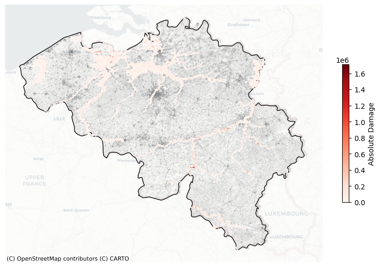
viz(damage_results)
fig, ax = plt.subplots(1,1,figsize=(7, 3))
sns.histplot(data=damage_results,x='damage',ax=ax)
#ax.set_ylim(0, 20000)
<Axes: xlabel='damage', ylabel='Count'>
9. Performing the Risk Assessment#
To do so, we need to select the return periods we want to include, and create a dictioniary as input. We will create this below.
return_periods = [2,5,10,50,100,200,500,1000]

hazard_dict = {}
for return_period in return_periods:
    hazard_map = xr.open_dataset(f"https://hazards-data.unepgrid.ch/global_pc_h{return_period}glob.tif", engine="rasterio")

    hazard_dict[return_period] = hazard_map.rio.clip_box(minx=country_bounds.minx.values[0],
                     miny=country_bounds.miny.values[0],
                     maxx=country_bounds.maxx.values[0],
                     maxy=country_bounds.maxy.values[0]
                    )
risk_results = DamageScanner(hazard_country, features, damage_curves, maxdam).risk(hazard_dict)
Risk Calculation: 100%|██████████| 8/8 [24:38<00:00, 184.80s/it]
[!IMPORTANT]
The Risk Assessment module in
DamageScanneris computationally intensive, especially when applied at a country level.
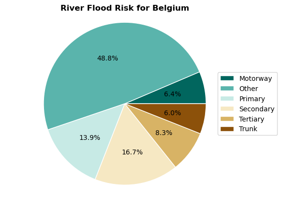
10. Visualize the Risk Assessment#
To understand the relative shares of each component of the system, we create a pie chart with the percentages of risk to each component.
risk_per_object = risk_results[['object_type','risk']].groupby('object_type').sum()
Here we set the colors.
colors = ['#8c510a','#d8b365','#f6e8c3','#c7eae5','#5ab4ac','#01665e'][::-1]
And create the figure
labels = [x.capitalize() for x in list(risk_per_object.index)]
sizes = risk_per_object.risk.values
pie = plt.pie(sizes,autopct='%1.1f%%', labeldistance=1.15, wedgeprops = { 'linewidth' : 1, 'edgecolor' : 'white' }, colors=colors);
plt.axis('equal')
plt.legend(loc = 'right', labels=labels,bbox_to_anchor=(1.15, 0.5),)
plt.title(f'River Flood Risk for {country_full_name}',fontweight='bold')
Text(0.5, 1.0, 'River Flood Risk for Belgium')