Systemic economic impacts of a transportation corridor failure

This notebook presents an example to demonstarte the systemic economic effects of a transportation corridor (road) failure in Belgium. We will follow the steps outlined below:

1. Data preparation:
   We will first download and create a network graph of the road network of Belgium. Next, we idealise the network into 11 nodes (corresponding to 11 NUTS-2 regions of Belgium) and 20 corridors b/w them.

2. Baseline distance b/w the regions:
   We estimate the distances between the nodes using shortest-path under a no disruption scenario.

3. Distance b/w the regions under disruption:
   For this example, we assume the road between Limburg (BE-22) and Liege (BE-33) is disrupted. Now we estimate the additional distances travelled b/w regions because of the disrupted corridor.

4. Input-Output Table aggregation:
   Next, we read the input-output table for Belgium and aggregate land-transportation sector into a value-added category. Also, we perform a basic input-output check.

5. System-level economic effects:
   We use a cost-push IO model (price model) to estimate the increased prices of goods which further leads to decreased consumption. Then, we employ a conventional leontief I-O (quantity model) to estimate the reduced production (output) across regions.

6. Results visualisation:
   Finally, we visualise the regional production losses across different NUTS-2 regions of Belgium.

1. Loading the required Packages and path directories

Show code cell source

Hide code cell source

# HIDE CODE
import geopandas as gpd
import numpy as np
import pandas as pd
# pd.set_option('future.no_silent_downcasting', True)

import damagescanner.download as download
import osmnx as ox
import networkx as nx
from shapely.ops import unary_union, linemerge
from shapely.geometry import Point


import matplotlib.pyplot as plt
import contextily as cx
import seaborn as sns
import matplotlib as mpl

from pathlib import Path
import os
import pyarrow
import openpyxl
from tqdm import tqdm

import warnings
warnings.filterwarnings("ignore", message="Geometry is in a geographic CRS")

Show code cell source

Hide code cell source

# HIDE CODE
base_path = Path(os.path.dirname(os.getcwd()) + "/data")
outpath = Path(os.path.dirname(os.getcwd()) + "/outputs")

2. Loading the Data

For the development of this notebook, we consider Belgium as the country of interest and roads for the Critical Infrastructure.

# NUTS 2016 Classification EU level
nuts_eu = gpd.read_file(base_path / 'NUTS_RG_03M_2016_4326.gpkg')

# NUTS-2 Regions of Belgium
nuts_be = nuts_eu[(nuts_eu['LEVL_CODE'] == 2) & (nuts_eu['CNTR_CODE'] == 'BE')].reset_index(drop = True)

Visualising the NUTS-2 Belgium regions

# Plotting
fig, ax = plt.subplots(figsize=(6,6))
nuts_be.plot(ax=ax, color = '#9A7AA0',  edgecolor='k', alpha = 0.5)
ax.axis('off')
plt.show()

Creating a points DataFrame

This will be useful in the later part of the notebook, where the points are assumed as nodes of the network.

# Point dataframe of NUTS-2 region of Netherlands
nuts_be_point = nuts_be.copy()
nuts_be_point['geometry'] = nuts_be.centroid

Downloading the roads of Belgium using DamageScanner.

# Downlaoding the openstreetmap data for the country of belgium
# The path contains the location of the downloaded pbf file
infrastructure_path = download.get_country_geofabrik('BEL') 

%%time

# Filtering the line types
roads = gpd.read_file(infrastructure_path, layer="lines")

# Filtering the DataFrame such that the highway columns is not None
roads = roads[roads["highway"].values != None]

CPU times: user 26 s, sys: 11.8 s, total: 37.8 s
Wall time: 1min 41s

roads.head()

	osm_id	name	highway	waterway	aerialway	barrier	man_made	railway	z_order	other_tags	geometry
0	75146	Rue de Thiribut	residential	NaN	NaN	NaN	NaN	NaN	3	NaN	LINESTRING (5.00314 50.57241, 5.0032 50.57244,...
1	195145	NaN	motorway_link	NaN	NaN	NaN	NaN	NaN	9	"destination"=>"Andenne;Bierwart;Mécalys;Ciney...	LINESTRING (5.06149 50.53069, 5.0604 50.53082,...
2	195314	NaN	motorway_link	NaN	NaN	NaN	NaN	NaN	9	"destination"=>"Hannut;Hingeon","destination:r...	LINESTRING (5.00917 50.53085, 5.01038 50.53093...
3	197574	NaN	trunk	NaN	NaN	NaN	NaN	NaN	8	"junction"=>"roundabout","lanes"=>"3","lit"=>"...	LINESTRING (4.52797 50.45663, 4.52794 50.45655...
4	197576	Rue du Bois des Loges	residential	NaN	NaN	NaN	NaN	NaN	3	"lanes"=>"2","lit"=>"yes","maxspeed"=>"30","su...	LINESTRING (4.96795 50.33742, 4.96782 50.33746...

3. Build a network graph of the roads

def build_graph(roads):

    """
    Function to create a network graph i.e., a network of nodes and edges from a DataFrame of roads
    ----------
    roads : GeoDataFrame with lines as geometries
    
    Returns
    -------
    G : network-x graph
        A graph of nodes and edges. The edges are the linestrings in the roads GeoDataFrame
    """

    roads = roads.copy()
    roads["length_m"] = roads.to_crs("EPSG:31370").geometry.length

    # Creating osmid column
    if "osm_id" not in roads.columns:
        roads["osm_id"] = range(len(roads))
        
    # Initiate a network x graph
    G = nx.Graph()
    
    for _, row in tqdm(roads.iterrows(), total = len(roads), desc = 'Building road graph'):
        start = row.geometry.coords[0]
        end   = row.geometry.coords[-1]
        
        # Adding edge to the graph
        G.add_edge(start, end,osmid = row["osm_id"], length_m = row["length_m"], geometry = row.geometry)
        
    # Only using the largest connected component 
    largest = max(nx.connected_components(G), key=len)
    G = G.subgraph(largest).copy()
    G.graph["crs"] = "EPSG:4326"
    
    return G

G = build_graph(roads)

Building road graph: 100%|██████████| 2207519/2207519 [01:10<00:00, 31217.87it/s]

4. Plotting the road network of belgium

print(f"Nodes: {G.number_of_nodes()}")
print(f"Edges: {G.number_of_edges()}")

# Plotting

# Extracting edges and creating a GeoDataFrame
edges = [(G[u][v]["geometry"]) for u, v in G.edges()]
edge_gdf = gpd.GeoDataFrame({"geometry": edges}, crs="EPSG:4326")

fig, ax = plt.subplots(figsize=(6, 6))
nuts_be.plot(ax=ax, color = '#9A7AA0',  edgecolor='k', zorder=1, alpha = 0.5)
edge_gdf.plot(ax=ax, color="white", linewidth=0.5, alpha = 0.5, zorder=2)
ax.axis('off')
plt.show()

Nodes: 639628
Edges: 756518

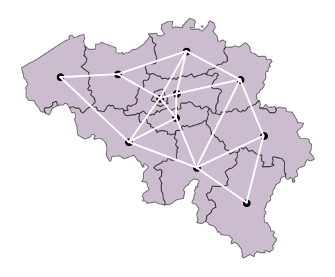
Next, we create a stylised representation of the road network between NUTS-2 regions of Belgium.

Adjacent matrices are square matrices of size equal to the number of nodes. Here, we consider the NUTS-2 regions as nodes. They contain the connectivity information between the regions. adj(i,j) = 1 if i and j has an edge between them; else 0.

# Adjacenct matrix for the network
adj_df = pd.read_excel(base_path /'adj_matrix.xlsx', index_col = 0)

Plotting the stylised road network of Belgium.

points = np.array([[pt.x, pt.y] for pt in nuts_be_point.geometry])
nuts_ids = nuts_be_point["NUTS_ID"].values

# Build a mapping from NUTS_ID to index
nuts_to_idx = {nid: i for i, nid in enumerate(nuts_ids)}

fig, ax = plt.subplots(figsize=(6,6))

# Plot the points
nuts_be.plot(ax=ax, color = '#9A7AA0',  edgecolor='k',  alpha = 0.5)
nuts_be_point.plot(ax=ax, color='k', markersize=50)

# Plot edges from adjacency DataFrame
for i, start in enumerate(adj_df.index):
    for j, end in enumerate(adj_df.columns):
        if adj_df.loc[start, end] == 1 and i < j:  # avoid double plotting
            x = [points[nuts_to_idx[start], 0], points[nuts_to_idx[end], 0]]
            y = [points[nuts_to_idx[start], 1], points[nuts_to_idx[end], 1]]
            ax.plot(x, y, color='white', lw=2)
            
ax.axis('off')
plt.show()

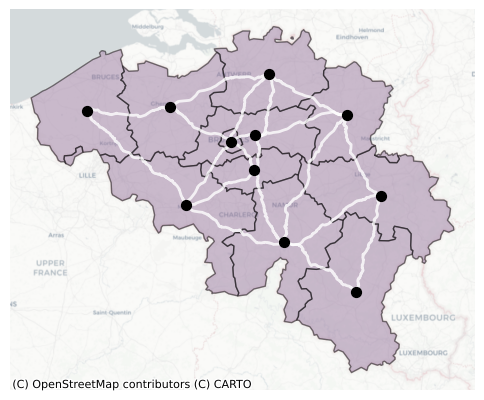
Now, we replace the straight lines with actual roads from the previously generated network graph.

def nearest_node(G, lon, lat):
    """
    Function to identify the closest node in a graph to the coordinates of interest
    ----------
    G : network-x graph
    lon: longitude of the coordinate of interest
    lat: latitude of the coordinate of interest
    
    Returns
    -------
    The closest node to the coordinates of interest
    """
    
    nodes = list(G.nodes)
    nodes_arr = np.array(nodes)
    dists = np.hypot(nodes_arr[:, 0] - lon, nodes_arr[:, 1] - lat)
    return nodes[np.argmin(dists)]

# Using points DataFrame to extract latitude and longitude
nuts_be_point['x'] = nuts_be_point.geometry.x
nuts_be_point['y'] = nuts_be_point.geometry.y

records = []


for i in range(len(nuts_be_point)):
    for j in range(len(nuts_be_point)):

        nutsid_1 = nuts_be_point.loc[i, 'NUTS_ID']
        nutsid_2 = nuts_be_point.loc[j, 'NUTS_ID']

        connection = adj_df.loc[nutsid_1, nutsid_2]

        if connection == 1:
            
            node_a = nearest_node(G, lon=nuts_be_point.loc[i,'x'],   lat=nuts_be_point.loc[i,'y'])
            node_b = nearest_node(G, lon=nuts_be_point.loc[j,'x'],   lat=nuts_be_point.loc[j,'y'])

            # Identifying the shorteest path
            path = nx.shortest_path(G, node_a, node_b, weight="length_m")

            # Converting multiple linestrings into a single line
            path_geoms = [G[u][v]["geometry"] for u, v in zip(path[:-1], path[1:])]
            single_line = linemerge(path_geoms)

            #  Appending to the list that stores the start, end and the adge information
            records.append({"nutsid_1": nutsid_1, "nutsid_2": nutsid_2, "geometry": single_line})

# Converting the edges to the DataFrame
roads_nuts2 = gpd.GeoDataFrame(records, geometry="geometry", crs=nuts_be_point.crs)

Creating a new graph with only NUTS-2 regions as nodes and the actual shortest path b/w them as edges.

G_nuts = build_graph(roads_nuts2)

Building road graph: 100%|██████████| 40/40 [00:00<00:00, 13441.13it/s]

Visualising the stylised network with actual roads.

fig, ax = plt.subplots(figsize=(6,6))

# NUTS-2 polygons
nuts_be.plot(ax=ax, color = '#9A7AA0',  edgecolor='k', zorder = 1, alpha = 0.5)\

# NUTS-2 points
nuts_be_point.plot(ax=ax, color='k', markersize=50, zorder = 3)

# Roads
edges_nuts = [(G_nuts[u][v]["geometry"]) for u, v in G_nuts.edges()]
edge_gdf_nuts = gpd.GeoDataFrame({"geometry": edges_nuts}, crs="EPSG:4326")
edge_gdf_nuts.plot(ax=ax, color="white", linewidth=2, alpha = 0.8, linestyle="-", zorder = 2)
cx.add_basemap(ax, source=cx.providers.CartoDB.Positron, crs=nuts_be.crs)

ax.axis('off')
plt.show()

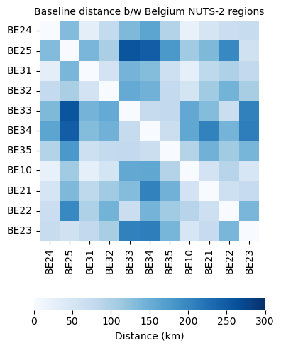
5. Baseline distance between the regions

# An empty DataFrame of size regions x regions to store the distance b/w them
distance_base = pd.DataFrame(index = nuts_ids, columns = nuts_ids)

for i in range(len(nuts_be_point)):
    for j in range(len(nuts_be_point)):

        # NUTS-IDs
        nutsid_1 = nuts_be_point.loc[i, 'NUTS_ID']
        nutsid_2 = nuts_be_point.loc[j, 'NUTS_ID']

        # Identifying the closest points in the graph
        node_a = nearest_node(G_nuts, lon=nuts_be_point.loc[i,'x'],   lat=nuts_be_point.loc[i,'y'])
        node_b = nearest_node(G_nuts, lon=nuts_be_point.loc[j,'x'],   lat=nuts_be_point.loc[j,'y'])

        # Distance in km
        dist_km = nx.shortest_path_length(G_nuts, node_a, node_b, weight="length_m")/1000
        distance_base.loc[nutsid_1, nutsid_2] = dist_km
        

Plotting a heatmap of distances b/w the regions

plt.figure(figsize=(5, 5))

distance_base = distance_base.astype(float)

ax = sns.heatmap(
    distance_base,
    cmap="Blues",
    vmin=0,
    vmax=300,
    square=True,
    cbar_kws={"label": "Distance (km)", "orientation": "horizontal","pad": 0.2,"fraction": 0.04})

ax.set_title("Baseline distance b/w Belgium NUTS-2 regions", fontsize = 10)

plt.tight_layout()
plt.show()

6. Distance between the regions under disruption

# The NUTS-2 IDs representing the start and end node of the failed corridor
province1 = 'BE22'
province2 = 'BE33'

def edge_removed_graph(G_fn, province1, province2):
    """
    Function to create a new network graph by removing the edge b/w two NUTS-2 regions
    ----------
    G_fn : network-x graph with all roads
    province1: The NUTS-2 IDs representing the start node of the failed corridor
    province2: The NUTS-2 IDs representing the end node of the failed corridor
    
    Returns
    -------
    an updated network graph with the edge b/w the nodes of interest removed
    """

    G_new = G_fn.copy()
    
    # The nearest nodes in the network
    node_a = nearest_node(G_new, lon=nuts_be_point[nuts_be_point['NUTS_ID'] == province1].reset_index(drop = True).loc[0,'x'],   lat=nuts_be_point[nuts_be_point['NUTS_ID'] == province1].reset_index(drop = True).loc[0,'y'])
    node_b = nearest_node(G_new, lon=nuts_be_point[nuts_be_point['NUTS_ID'] == province2].reset_index(drop = True).loc[0,'x'],   lat=nuts_be_point[nuts_be_point['NUTS_ID'] == province2].reset_index(drop = True).loc[0,'y'])

    # Remove the edge
    G_new.remove_edge(node_a, node_b)
    
    return G_new

# Revised graph with failed edge removed
G_nuts_disrupt = edge_removed_graph(G_nuts, province1, province2)

Visualising the failed corridor

fig, ax = plt.subplots(figsize=(6,6))

# Plot the points

nuts_be.plot(ax=ax, color = '#9A7AA0',  edgecolor='k', zorder = 1, alpha = 0.5)
nuts_be_point.plot(ax=ax, color='k', markersize=50, zorder = 4)

# plot it
edges_nuts = [(G_nuts[u][v]["geometry"]) for u, v in G_nuts.edges()]
edge_gdf_nuts = gpd.GeoDataFrame({"geometry": edges_nuts}, crs="EPSG:4326")
edge_gdf_nuts.plot(ax=ax, color="r", linewidth=2, alpha = 0.8, linestyle="-", zorder = 2)

edges_nuts_d = [(G_nuts_disrupt[u][v]["geometry"]) for u, v in G_nuts_disrupt.edges()]
edge_gdf_nuts_d = gpd.GeoDataFrame({"geometry": edges_nuts_d}, crs="EPSG:4326")
edge_gdf_nuts_d.plot(ax=ax, color="white", linewidth=2, alpha = 1, linestyle="-", zorder = 3)


cx.add_basemap(ax, source=cx.providers.CartoDB.Positron, crs=nuts_be.crs)

ax.axis('off')
plt.show()

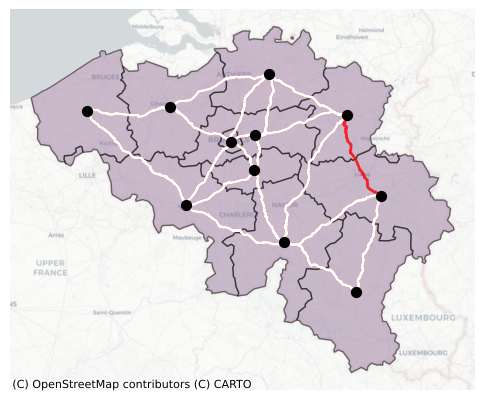
Since a corridor is removed, the shortest distance b/w some of the regions might increase. Next, we estimate the increased distances b/w the regions.

# An empty DataFrame to hold the distance b/w regions after disruption
distance_disrupt = pd.DataFrame(index = nuts_ids, columns = nuts_ids)

for i in range(len(nuts_be_point)):
    for j in range(len(nuts_be_point)):

        # NUTS-ID
        nutsid_1 = nuts_be_point.loc[i, 'NUTS_ID']
        nutsid_2 = nuts_be_point.loc[j, 'NUTS_ID']

        # Nearest nodes in the network graph
        node_a = nearest_node(G_nuts_disrupt, lon=nuts_be_point.loc[i,'x'],   lat=nuts_be_point.loc[i,'y'])
        node_b = nearest_node(G_nuts_disrupt, lon=nuts_be_point.loc[j,'x'],   lat=nuts_be_point.loc[j,'y'])

        # Distance in km
        dist_km = nx.shortest_path_length(G_nuts_disrupt, node_a, node_b, weight="length_m")/1000
        distance_disrupt.loc[nutsid_1, nutsid_2] = dist_km

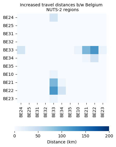
# Increased distance between regions
delta_distance = distance_disrupt - distance_base

Plotting a heatmap of increased distance between the regions

plt.figure(figsize=(5, 5))

delta_distance = delta_distance.astype(float)

ax = sns.heatmap(
    delta_distance,
    cmap="Blues",
    vmin=0,
    vmax=200,
    square=True,
    cbar_kws={"label": "Distance (km)", "orientation": "horizontal","pad": 0.2,"fraction": 0.04})

ax.set_title("Increased travel distances b/w Belgium \n NUTS-2 regions", fontsize = 10)

plt.tight_layout()
plt.show()

7. Input-Output table aggregation

The IO table above is an aggregated IO table for the NUTS-2 regions of Belgium.

• The sector ‘p’ represents products i.e., primarily sectors that produce physical goods (e.g., agricultural, manufacturing, minining).

• The sector ‘s’ represents service-based sectors.

• The sector ‘t’ represents the sector of land-transportation (H49 per NACE-2).

# Reading the IO table for Belgium
io = pd.read_excel(base_path / 'io_belgium.xlsx', index_col = [0,1], header = [0,1])

We aggregate all transport sectors into one single row (value added by land-transport) and single column (final demand for land-transport sector).

# Transport value-added
tva = io.loc[( nuts_ids,'t'),:].sum(axis = 0)

# Dropping all 't' sector rows
io = io.drop(index ='t', level=1)

# Adding the value-added transport column again
io.loc[('R','VA_t'), :] = tva

# Transport final demands
tfd = io.loc[:,( nuts_ids,'t')].sum(axis = 1)

# Dropping all 't' sector columns
io = io.drop(columns ='t', level=1)

# Adding the value-added transport column again
io.loc[:, ('R','FD_t')] = tfd

IO Check: Sum of rows (Output) equals sum of columns (Outlays).

io_check = pd.DataFrame(columns = ['rowsum', 'colsum'])

io_check['rowsum'] = io.sum(axis = 0)
io_check['colsum'] = io.sum(axis = 1)

io_check['diff'] = io_check['rowsum'] - io_check['colsum']

# Converting annaul IO flows to daily flows
io_daily = io/365

8. System-level economic effects

The increased travel distance between the origin and destinations primarily propagates into the economy via (a) Shortage effect - Products not available in time for continued production activities and (b) Price effect - The price of goods increases due to increased distances for transporting goods from one region to other.

For this example, delays caused by the corridor failure are expressed in hours, primarily because of smaller geography and more re-reouting options available. Hence, we do not consider the shortage effects. However, shortage effects can be crucial when regions are inaccessible or delays are significantly large, as in the case of Suez canal blockage.

io.head()

	r	BE10		BE21		BE22		BE23		BE24		...	BE32	BE33		BE34		BE35		R
	sd	p	s	p	s	p	s	p	s	p	s	...	s	p	s	p	s	p	s	FD	exp	FD_t
BE10	p	52.797997	169.068634	130.508057	92.403465	60.889435	43.626633	114.656288	68.264587	41.833893	73.736481	...	55.379299	62.748283	55.710030	15.259095	11.886464	17.164982	24.522854	3790.647461	3332.961182	62.699004
	s	810.859680	26420.080078	2388.069580	6036.488770	309.333832	1215.953979	602.770935	2433.725098	175.310715	2581.921387	...	2333.582031	684.252686	2161.123779	82.515457	324.608032	103.369423	697.338135	52434.562500	15736.668945	1696.505419
BE21	p	762.007507	1893.024658	12033.195312	3364.795166	1763.075195	811.292114	3706.054443	1643.714111	1364.426636	1704.064941	...	761.455383	1583.401855	895.615173	132.257812	76.832603	138.379105	157.111465	28321.802734	17103.281250	1462.361204
	s	477.225769	4812.578125	9982.744141	18079.138672	574.655457	1236.322388	929.046265	1922.102295	177.873260	1763.003174	...	1423.620117	352.594543	1417.108643	37.778591	226.722488	51.961910	533.839539	51692.222656	4190.382812	2383.296903
BE22	p	79.502617	211.340836	450.302429	304.396393	264.505524	238.780060	394.414520	264.914520	181.066040	175.944626	...	175.418854	256.165588	185.833847	32.977226	22.460728	45.922188	46.857548	5869.531738	6200.022949	59.759147

5 rows × 25 columns

Preparing arrays for Input-Ouput analysis.

# Intermediate consumption
Z = io_daily.loc[io.index.get_level_values(0) != 'R', io.columns.get_level_values(0) != 'R']

# Final consumption
fd = (io_daily.loc[io.index.get_level_values(0) != 'R', io.columns.get_level_values(0) == 'R'].sum(axis = 1).to_frame(name = 'FD'))

# Output = Intermediate consumption + Final consumption
x = (Z.sum(axis=1) + fd.sum(axis=1)).to_frame(name = 'x')

# Technical coefficients
A = pd.DataFrame(0, index = Z.index, columns = Z.columns, dtype = 'float64')

# Calculating technical coefficients
for i in range(len(x)):
    A.iloc[:,i] = Z.iloc[:,i] / x.iloc[i,0]

# Flattening final demand and Ouptu arrays
fd_array =fd.values.flatten()
x_array = x.values.flatten()

# Converting dataframe to numpy array
A_array = A.values

# Value added array
# This is vector equals the shape number of sectors (11 regions x 2 sectors) , number of va categories
# We have three VA categories VA, Imports and VA by land tranport

va = io_daily.loc[io.index.get_level_values(0) == 'R', io.columns.get_level_values(0) != 'R'].T.to_numpy()

# Dividing the va columns with output to determine va to output ratio for each category
va_x = va/x_array[:,None]

# Sum across the ratio to determine the total va to output ratio
va_x_sum = va_x.sum(axis =1)

Due to the increased travel distance between the NUTS-2 regions, the logistic costs of inputs increase. As a result, the price of outputs produced also increases. This can be quantified using Cost-Push IO Model or the Leontief price Model. Further, consumers reduce consumption due to higher prices. Reduced consumption also leads to reduced production upstream.

Cost-push IO model is given by prices = (leontief inverse)’ x (va/x). Refer Miller&Blair(2009), Chapter 2 for more details.

#Leontief inverse
leontief_inverse = np.linalg.inv(np.eye(len(x_array)) - A_array)

# Leontief inverse transpose
leontief_inv_trans =  np.transpose(leontief_inverse)

Calculating base prices i.e., unit vector check

# Base prices
base_price = leontief_inv_trans@ va_x_sum 
base_price

array([1.00000001, 1.00000003, 1.00000001, 1.00000001, 0.99999998,
       1.00000003, 0.99999995, 1.00000004, 0.99999997, 1.00000003,
       0.99999997, 0.99999998, 1.        , 1.00000003, 1.00000002,
       0.99999998, 1.        , 1.00000002, 1.00000003, 0.99999996,
       1.00000001, 0.99999998])

We estimate the ratio of increased distance b/w pre and post disruption across NUTS-2 regions. 1 indicates the flow is unaffected by the disruption. Next, we calculate the flow-weighted increase of this multiplier only for the product sectors. This multipler is then used to increase the value-added cost and the new prices are estimated.

# Ratio of distance travelled in the disrupted scenario to the disatnce travelled in the baseline scenario
ratio_dist_disrupt = distance_disrupt.replace(0,1) / distance_base.replace(0,1)

# product flows
p_flow = io_daily.loc[io.index.get_level_values(1) == 'p', io.columns.get_level_values(1) == 'p']

p_flow.index = p_flow.index.droplevel(1)
p_flow.columns = p_flow.columns.droplevel(1)

#### Weighted ratios
ratio_p_weighted = ratio_dist_disrupt*p_flow

#### Divide the flows
va_t_multiplier = (ratio_p_weighted.sum() / p_flow.sum()).to_numpy()

We assume price shocks affect product sectors and not service sectors. Service economic flows have less dependence on physical transport networks compared to products.

Now, we estimate the increased prices.

# Initialsiing a zero array to the length of all sectors
price_shock = np.ones(len(va_t_multiplier)*2)

# Price shocks only to the product sector
price_shock[::2] = va_t_multiplier

# Price shock is multiplied to the third column of value added which is the cost w.r.t to transport
va_x_revised = va_x.copy()
va_x_revised[:,2] *= price_shock

# Revised va_x_sum
va_x_sum_revised = va_x_revised.sum(axis =1)

# Increased prices
increased_price = leontief_inv_trans@ va_x_sum_revised
increased_price

array([1.00029234, 1.00006241, 1.00061997, 1.00008895, 1.0036805 ,
       1.00011696, 1.0003741 , 1.00008829, 1.00041272, 1.00006979,
       1.00029948, 1.00010032, 1.00015446, 1.00008084, 1.00032213,
       1.0000955 , 1.00985105, 1.00012331, 1.00120859, 1.00008614,
       1.00028291, 1.00009238])

The increased prices are translated to corresponding reduction in consumption. We assume that the demand curve follows dP/dQ = -1 i.e., dP increase in price will lead to dQ decrease in quantity. FD_price_effect = (FD_BASE x -dP) + FD_BASE.

# final demands corrected for price effect
fd_price = (fd_array*(increased_price-1)*-1)+fd_array

Finally, we estimate the new production (or output) required for the reduced demand using a Leontief IO (quantity model).

# X = L-1 x fd
x_price = leontief_inverse@fd_price

# Reduction in output
del_x_price = x_array - x_price

# Creating a new column in the output DataFrame
x['output_loss'] = del_x_price

# Aggregation regioanlly
x_groupued = x.groupby(level =0).sum()

# Merging it to the geodataframe
nuts_be_region = nuts_be.set_index('NUTS_ID')
nuts_price = gpd.GeoDataFrame(pd.merge(x_groupued, nuts_be_region , how = 'inner', left_index=True, right_index = True))

total_output_loss = nuts_price.output_loss.sum()

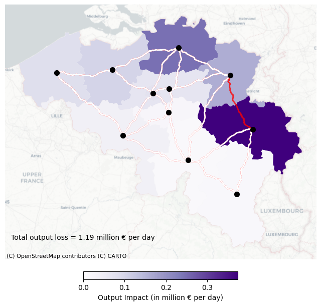
Results visualisation

Now, we plot the production decrease in each NUTS-2 region of Belgium.

fig, ax = plt.subplots(figsize=(8,8))

# Plot the points
cmap = plt.cm.Purples
norm = mpl.colors.Normalize(vmin=0, vmax = nuts_price.output_loss.max())

# The nuts dataframe which also contains the information about output loss in the region
nuts_price.plot(ax = ax, column = 'output_loss', cmap = cmap, norm = norm)
nuts_be_point.plot(ax=ax, color='k', markersize=50, zorder = 4)

# Plotting the failed raod
edges_nuts = [(G_nuts[u][v]["geometry"]) for u, v in G_nuts.edges()]
edge_gdf_nuts = gpd.GeoDataFrame({"geometry": edges_nuts}, crs="EPSG:4326")
edge_gdf_nuts.plot(ax=ax, color="r", linewidth=2, alpha = 0.8, linestyle="-", zorder = 2)

# Plotting other roads
edges_nuts_d = [(G_nuts_disrupt[u][v]["geometry"]) for u, v in G_nuts_disrupt.edges()]
edge_gdf_nuts_d = gpd.GeoDataFrame({"geometry": edges_nuts_d}, crs="EPSG:4326")
edge_gdf_nuts_d.plot(ax=ax, color="white", linewidth=2, alpha = 1, linestyle="-", zorder = 3)

# A text box to indicate total loss
ax.text(0.02, 0.1, f'Total output loss = {total_output_loss:.2f} million € per day', transform=ax.transAxes, fontsize=10, verticalalignment='top',zorder=10)

cx.add_basemap(ax, source=cx.providers.CartoDB.Positron, crs=nuts_be.crs)

sm = mpl.cm.ScalarMappable(norm=norm, cmap=cmap)
sm.set_array([])

cbar = fig.colorbar(sm,ax=ax,orientation='horizontal',fraction=0.025,   pad=0.04)
cbar.set_label('Output Impact (in million € per day)')

ax.axis('off')
plt.savefig(os.path.join(outpath, "systemic_impact.png"), dpi=300)
plt.show()