Cost-Benefit Analysis

In this example, we develop a stylised example template for Cost-benefit Analysis (CBA).

CBA involves prior estimation of the Expected Annnual direct Damages (EAD) and Expected Annual indirect Economic Losses (EAEL) with and without the implementation of an adaptation option. These losses are estimated over a set of consecutive years or in most cases at specific time horizons. For example - EAD and EAEL might be estimated for a given baseline year (e.g. 2025) and for future years for which climate scenario-based hazard maps might be created (e.g. 2050, 2080 SSP3 7.0).

CBA also requires inputs of the initial investment costs of the adaptation option, and its maintenance costs (recurrent and periodic).

Further inputs include the timeline of the CBA assessment and discount rates. Economic GPD growth rates might also be needed to project future EAELs.

The outputs of this analysis are the benefits (avoided damages and losses over time), the costs and the Benefit-Cost Ratio (BCR).

\[\text{Benefits} = (\text{EAD}_{\text{without adaptation}} - \text{EAD}_{\text{with adaptation}}) + (\text{EAEL}_{\text{without adaptation}} - \text{EAEL}_{\text{with adaptation}})\]

\[\text{Costs} = \text{Initial investment} + \text{Maintenance over time}\]

\[\text{Benefit-Cost Ratio (BCR)} = \frac{\text{Discounted Benefits}}{\text{Discounted Costs}}\]

import os
from pathlib import Path
import pandas as pd
import numpy as np
import warnings
import matplotlib.pyplot as plt
from cba.cba_functions import *

warnings.simplefilter("ignore")
base_path = Path(os.path.dirname(os.getcwd()) + "/data")
outpath = Path(os.path.dirname(os.getcwd()) + "/output")

1. Setup and Data Acquisition

Read CBA model parameters

loss_id_column = "id"
dimension_column = "length"
loss_columns = ["EAD", "EAEL"]
cost_columns = ["initial_investment", "periodic_maintenance", "recurrent_maintenance"]
year_column = "year"
options_columns = ["option", "hazard"]

parameter_df = pd.read_csv(base_path / "cba_parameters.csv")
parameters = parameter_df.set_index("parameter").to_dict()["value"]
st_y = int(parameters["start_year"])
en_y = int(parameters["end_year"])
d_r = float(parameters["discount_rate"])
apply_gdp_series = parameters["apply_gdp_timeseries"]
apply_gdp_fixed_rate = parameters["apply_fixed_gdp_growth"]
gdp_r = float(parameters["gdp_rate"])

timeseries = np.arange(st_y, en_y + 1, 1)

Read damages and losses without adaptation and convert to timeseries

noadapt_df = pd.read_csv(base_path / "without_adaptation_losses.csv")
noadapt_df = estimate_risk_time_series(
    noadapt_df, ["hazard"], loss_columns, "year", st_y, en_y
)

Read damages and losses with adaptation and convert to timeseries

adapt_df = pd.read_csv(base_path / "with_adaptation_losses.csv")
adapt_df = estimate_risk_time_series(
    adapt_df, ["hazard", "option"], loss_columns, "year", st_y, en_y
)

Merge the loss DataFrames and estimate avoided losses

noadapt_df.rename(
    columns=dict([(lc, f"{lc}_noadapt") for lc in loss_columns]), inplace=True
)
adapt_df.rename(
    columns=dict([(lc, f"{lc}_adapt") for lc in loss_columns]), inplace=True
)
n_idx_cols = [c for c in noadapt_df.columns.values.tolist() if c not in loss_columns]
a_idx_cols = [c for c in adapt_df.columns.values.tolist() if c not in loss_columns]

adapt_df = pd.merge(
    adapt_df, noadapt_df, how="left", on=list(set(a_idx_cols).intersection(n_idx_cols))
)
for lc in loss_columns:
    adapt_df[f"avoided_{lc}"] = adapt_df[f"{lc}_noadapt"] - adapt_df[f"{lc}_adapt"]

2. Economic Loss Analysis

Project the Avoided Economic losses by some GDP change factor, if needed

gr_f = []
if apply_gdp_series == "TRUE":
    gr_f = pd.read_csv(base_path / "gdp_timeseries.csv")
    gr_f = list(gr_f.itertuples(index=False, name=None))
    gr_f = calculate_growth_rate_factor(gr_f, st_y, en_y)
elif apply_gdp_fixed_rate == "TRUE":
    gr_f = calculate_growth_rate_factor(gdp_r, st_y, en_y)

if len(gr_f) > 0:
    gr_f = pd.DataFrame(gr_f, columns=[year_column, "gdp_factor"])
    adapt_df = pd.merge(adapt_df, gr_f, how="left", on=[year_column])
    adapt_df["avoided_EAEL"] = adapt_df["avoided_EAEL"] * adapt_df["gdp_factor"]
    adapt_df.drop("gdp_factor", axis=1, inplace=True)

3. Cost-Benefit Calculation

Estimate the adaptation cost timeseries

cost_df = pd.read_csv(base_path / "adaptation_options_and_costs.csv")
cost_df = estimate_adaptation_cost_time_series(
    cost_df, ["option", "hazard", "adapt_cost_uom"], start_year=st_y, end_year=en_y
)

Merge the adaptation losses with the adaptation costs to estimate the benefits and cost

adapt_df = pd.merge(
    adapt_df, cost_df, how="left", on=options_columns + [year_column]
).fillna(0)
adapt_df["benefit"] = adapt_df[[f"avoided_{lc}" for lc in loss_columns]].sum(axis=1)
adapt_df["cost"] = adapt_df[cost_columns].sum(axis=1)
adapt_df["cost"] = adapt_df["cost"] * adapt_df[dimension_column]

Do the discounting of the benefits and the costs based on the discount rate

dis_series = calculate_discounting_rate_factor(
    discount_rate=d_r, start_year=st_y, end_year=en_y, maintain_period=1.0
)
dis_df = pd.DataFrame(
    list(zip(timeseries, dis_series)), columns=[year_column, "discount_rate"]
)
adapt_df = pd.merge(adapt_df, dis_df, how="left", on=[year_column])
adapt_df["benefit_pv"] = adapt_df["benefit"] * adapt_df["discount_rate"]
adapt_df["cost_pv"] = adapt_df["cost"] * adapt_df["discount_rate"]

4. Synthesis and Results

Estimate the added benefits, costs, and BCR summed over the timeseries

sum_columns = ["benefit", "cost", "benefit_pv", "cost_pv"]
df = (
    adapt_df.groupby([loss_id_column] + options_columns)
    .agg(dict([(c, "sum") for c in sum_columns]))
    .reset_index()
)
df["BCR"] = df["benefit_pv"] / df["cost_pv"]
df

	id	option	hazard	benefit	cost	benefit_pv	cost_pv	BCR
0	1	flood wall	flood	32627.951377	4875.0	9335.697257	2863.302085	3.260465
1	1	swales	flood	20718.844610	1625.0	5949.529544	954.434028	6.233568
2	2	flood wall	flood	2238.576048	975.0	660.842549	572.660417	1.153987
3	2	swales	flood	809.483236	325.0	254.502424	190.886806	1.333264

Save the final results

df.to_csv(outpath / "CBA_result.csv", index=False)

5. Validation and Visualisation

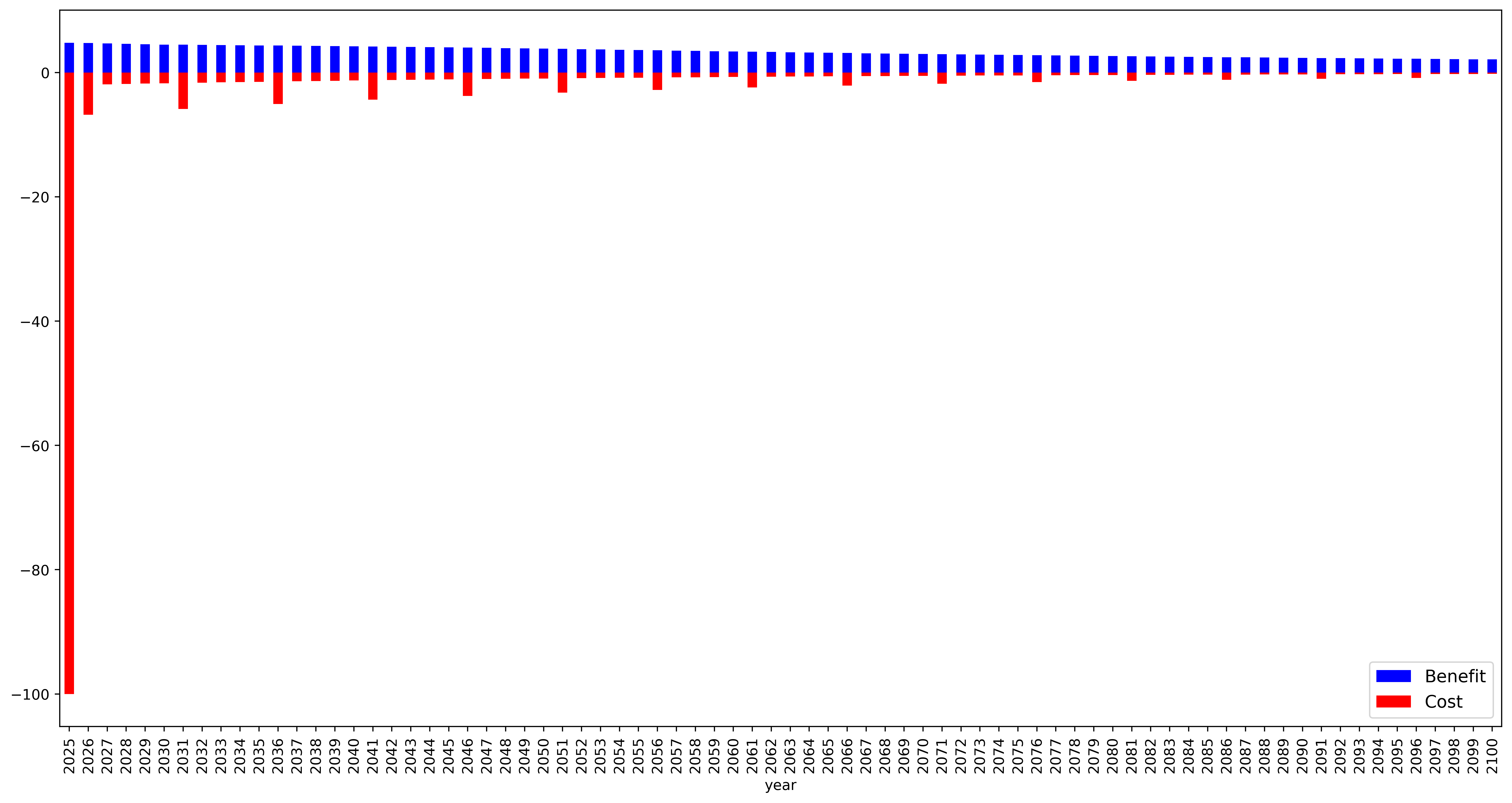
Test - Plot of Benefit and Cost timeseries with or without discounting

fig, ax = plt.subplots(1, 1, figsize=(18, 9), dpi=500)
test_df = adapt_df[(adapt_df["id"] == 2) & (adapt_df["option"] == "swales")]
test_df["cost"] = -1.0 * test_df["cost"]
test_df.plot.bar(ax=ax, x=year_column, y="benefit", color="b")
test_df.plot.bar(ax=ax, x=year_column, y="cost", color="r")
ax.legend(["Benefit", "Cost"], loc="lower right", fontsize=12)

<matplotlib.legend.Legend at 0x15c4dba90>

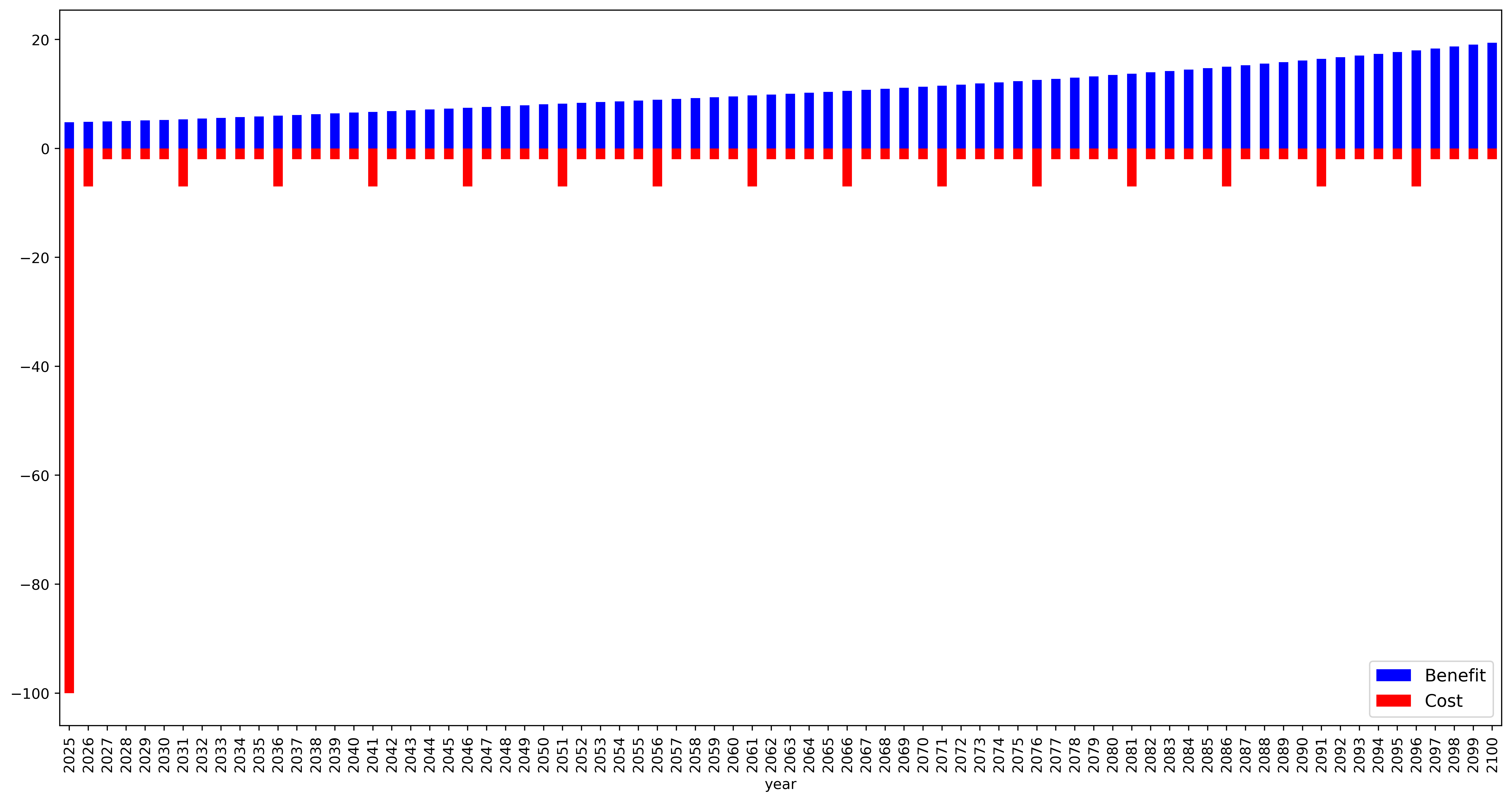
fig, ax = plt.subplots(1, 1, figsize=(18, 9), dpi=500)
test_df = adapt_df[(adapt_df["id"] == 2) & (adapt_df["option"] == "swales")]
test_df["cost_pv"] = -1.0 * test_df["cost_pv"]
test_df.plot.bar(ax=ax, x=year_column, y="benefit_pv", color="b")
test_df.plot.bar(ax=ax, x=year_column, y="cost_pv", color="r")
ax.legend(["Benefit", "Cost"], loc="lower right", fontsize=12)

<matplotlib.legend.Legend at 0x15cf5b460>